
This article is the third part of a three part series on the PERF (linux-tools) performance measurement and profiling system for Linux.
- Part 1 demonstrates how to use PERF to identify and analyze the hottest execution spots in a program. Part 1 covers the basic PERF commands, options and software performance events.
- Part 2 introduces hardware performance events and demonstrates how to measure hardware events across an entire application.
- Part 3 uses performance event sampling to identify and analyze hot spots within an application program.
Each article builds on the usage and background information presented in the previous articles. So, if you’ve arrived here through a Web search, please scan the preceding articles for background. All articles use the same two example programs:
- Naive: Naive matrix multiplication program (textbook algorithm).
- Interchange: An improved matrix multiplication program (loop nest interchange algorithm).
The textbook algorithm has known performance issues due to its memory access pattern. The loop nest interchange algorithm has a different access pattern which reads/writes data more efficiently.
Author: P.J. Drongowski
Introduction
This article demonstrates PERF performance counter sampling mode. If you have read the first two parts of this tutorial series, then you already have much of the basic background for performance counter sampling. Instead of using the software CPU clock to sample your program with perf record as shown in Part 1, use one (or more) of the hardware performance events that are discussed in Part 2.
If you didn’t read parts 1 and 2, don’t worry. I illustrate the analytical process along with many fine points about performing arithmetic on samples and sampling accuracy. The running example is the same (matrix multiplication) although the matrix size is larger (1000 by 1000 square matrices instead of 500 by 500). I increased the matrix size in order to put more stress on the memory subsystem and to increase program run time.
Sampling period and sampling frequency
Before diving into the details, here are a few ideas and terms to keep in mind.
Performance counter sampling is a statistical measurement technique. PERF selects the samples and stores them in a file named “perf.data“. After sample collection, the individual samples are aggregated during post-processing. The final statistics and distribution of samples give us insight into program behavior and performance.
PERF selects each sample such that we obtain a statistically representative result. The conventional method for sample selection is a fixed sampling period, which is the number of events which occur between samples. Each event type (e.g., cycles, instructions, etc.) to be collected has its own sampling period. Some profilers randomize the sampling period; PERF does not.
With a fixed sampling period, each sample for a given event has a specific weight which is equal to the number of events in the sampling period. For example, when we measure retired instructions with a sampling period of 100,000, each sample represents 100,000 retired instructions. We can easily convert the number of retired instruction samples to the (estimated) raw number of retired instructions by multiplying the number of samples times the sampling period:
    Number of instructions =
        (Sampling period) * (Number of instruction samples)
In addition to a fixed sampling period, PERF implements an alternative method for sample selection called “sampling frequency.” The sampling frequency is specified as a samples per second rate. It is the average rate and is not fixed. PERF dynamically adjusts the hardware-level sampling period to achieve the goal frequency. Adjustments are recorded in the profile data file. Real world workload behavior varies during execution so you should expect adjustments.
My personal experience is with fixed sampling periods. I like the property where the weight is the same for each and every sample for a given event and its sampling period. To my mind, it makes it easier to normalize weights and to perform arithmetic on event sample quantities. The data and discussion below use fixed sampling periods exclusively.
Example workload: matrix multiplication
We are measuring the same example programs as parts 1 and 2 except that matrix size is increased from 500 by 500 square matrices to 1000 by 1000 square matrices. This simple change substantially increases run time due to a larger number of arithmetic operations (larger matrices mean more instructions to execute) and due to greater stress on the Raspberry Pi 2 memory subsystem. In parts 1 and 2, large portions of the relatively small operand matrices fit into L2 cache. The larger matrices easily exceed the L2 cache size and have a much larger virtual memory working set. The larger working set and longer memory stride cause even more data translation look-aside buffer (dTLB) misses.
The naive matrix multiplication program uses the standard textbook algorithm. The improved matrix multiplication program implements the loop nest interchange algorithm. I named these programs and test cases “large_naive” and “large_interchange,” respectively, to denote the differences in algorithm and matrix size.
The test platform is a Raspberry Pi 2 (900MHz ARMv7 Cortex-A7 quad-core processor) with 1GByte of primary memory. The operating system is Raspbian Wheezy 3.18.9-v7+. You should obtain similar results on x86 and other architectures, modulo processor-specific cache and translation look-aside buffer (TLB) sizes. The techniques demonstrated here can be applied on any processor, not just ARMv7.
The following table summarizes elapsed time and performance event measurements made using PERF counting mode. The loop nest interchange algorithm is twice as fast as the naive algorithm due to its efficient memory access pattern.
| Event or metric | large_naive | large_interchange |
|---|---|---|
| Elapsed time | 42.72 seconds | 19.39 seconds |
| instructions | 9,202,412,724 | 9,190,021,947 |
| cycles | 38,404,339,752 | 17,384,679,496 |
| cache-references | 2,121,045,751 | 3,068,419,167 |
| cache-misses | 992,217,145 | 72,674,306 |
| LLC-loads | 1,979,027,672 | 148,265,528 |
| LLC-load-misses | 68,018,035 | 64,436,897 |
| dTLB-load-misses | 930,209,535 | 1,117,864 |
| branches | 1,029,438,167 | 1,022,563,043 |
| branch-misses | 6,101,021 | 4,760,643 |
Both programs execute approximately the same number of instructions. Due to the shorter run time, large_interchange takes (roughly) half the number of processor cycles as large_naive. Even though large_interchange makes more cache references, it makes better use of the cache and has fewer cache misses. large_interchange has substantially fewer dTLB misses because it has a smaller dynamic page working set.
The next table presents the ratios and per thousand instruction (PTI) rates for the two programs. Rates and ratios provide more intuitive insight into program behavior and efficiency than raw event counts. Instructions per cycle (IPC) for large_interchange is twice the IPC value for large_naive reflecting the 2x difference in execution time.
| Ratio or rate | large_naive | large_interchange |
|---|---|---|
| IPC | 0.24 | 0.53 |
| Cache miss ratio | 0.47 | 0.02 |
| Cache miss rate PTI | 107.82 | 7.91 |
| LLC load miss ratio | 0.03 | 0.43 |
| LLC load miss rate PTI | 7.39 | 7.01 |
| dTLB load miss rate PTI | 101.08 | 0.12 |
| Branch mispredict ratio | 0.01 | <0.01 |
| Branch mispred rate PTI | 0.66 | 0.52 |
The change in cache miss rate PTI and dTLB miss rate PTI is noteworthy. The innermost loop in both programs is nine instructions long. The cache and dTLB miss rates PTI for large_naive indicate a cache and/or dTLB miss on nearly every loop iteration.
Admittedly, matrix multiplication is often regarded as a “toy” performance analysis example. These rates and ratios, however, provide a rough guideline for acceptable and unacceptable event rates and ratios. Developers are often perplexed when they encounter rates and ratios in real world practice, specifically, “When and at what level does a metric indicate a performance issue?” Comparing the measurements for known bad vs. known good program behavior helps us identify values that signal the presence of a performance issue to be mitigated through tuning. Manufacturers rarely provide this kind of information even though they benchmark a processor design extensively during hardware development. (Sigh.)
Collect profile data
The perf record command collects event samples and stores them in a file. By default, PERF stores the samples in a file name “perf.data“. Reporting commands like perf report read sample data from perf.data by default. You may specify the output file name explicitly by including the -o (--output) option on the command line. The following command collects samples for the hardware cpu-cycles event.
perf record -e cpu-cycles -c 100000 ./large_naive
The -c (--count) command line option above specifies a fixed sampling period of 100,000 cpu-cycles. The -F (--freq) command line option specifies the sampling frequency in terms of events per second. If you do not specify the sampling period or sampling frequency on the command line, PERF uses a default rate of 1000 samples per second.
As described in part 2 of this series, the underlying processor has a small number of hardware event counters in each core. The Broadcom BCM 2836 in the Raspberry Pi 2 has four ARM Cortex-A7 cores and each core has four performance counters. You may measure up to four different events in a single run. Check the technical reference manual for the processor in your test platform for details about available performance events and counters.
This last paragraph is a simplification for purposes of this tutorial. More events per run can be collected through counter multiplexing. Also, counters can be configured for system-wide and per-core operation. These features are advanced topics and are beyond an introductory article.
When looking for the hottest spots in an application, you may choose to profile your program using cpu-cycles because the cpu-cycles event is a measure of time just like the cpu-clock software event. Either kind of event will get you to the same result — a profile showing where the program spends most of its execution time. The cpu-cycles event can provide higher resolution, but high resolution comes at a cost. (More about all of this in a moment.)
Hardware event sampling is performed in the following way. PERF configures the hardware performance counters to count the selected events. It also configures each counter to generate an interrupt after the occurrence of the number of events specified by the sampling period. PERF starts the counters and launches the workload. When the sampling period expires for a counter, it generates an interrupt. PERF then reads the restart program counter value from the interrupt stack and writes the PC value (and other information) to a sample buffer. PERF writes the sample buffer to the profile data file when the buffer is full. Finally, PERF re-arms (no pun intended) the performance counter and sets the sampling period after making any needed adjustments for sampling frequency. This whole process continues until the workload completes and PERF disables the hardware performance counters.
Although you do not need to fully understand this process, you should be aware of two important, practical points.
- Profiling tools like perf report need to associate each event sample with a program instruction or line of source code. Ideally, this is the actual instruction or line of source that caused the event which triggered the sampling interrupt. The restart PC does not usually point to the culprit and it provides only an approximation location for the event within the program.
- Sampling interrupts occur and are handled on the same core as the workload. Thus, workload behavior is changed by the measurement process (shades of Heisenberg) and interrupt handling robs CPU time from the workload. Expect a longer elapsed time due to measurement overhead when sampling.
The first concern is mitigated on processor architectures that support precise attribution of a performance event to the instruction which actually caused the event. On Intel x86 processors, this facility is known as “Precise Event Based Sampling” or “PEBS.” On AMD x86 processors, precise attribution is provided by “Instruction Based Sampling” or “IBS.” PERF supports both.
The second concern — sampling interrupts and overhead — may be alleviated by careful selection of sampling period (or sampling frequency).
Choosing the sampling period
We need to trade off several factors when choosing the sampling period for an event.
- Statistical accuracy and resolution
- Perturbations to workload behavior
- Overhead
- Relative event frequency (low vs. high)
- Ease of computation
I’ll first discuss each of these factors before describing my choice for this article (100,000 events in each fixed period).
Sampling is a statistical process, so in general, accuracy increases when more samples are taken. Resolution (the number of significant digits in the result) also improves when more samples are taken. We need to collect enough samples to have a statistically representative result from which we can reliably draw inferences about program behavior.
One way to increase sample volume is to decrease the sampling period. More event samples are collected when the period is shorter; there are fewer individual events between samples so more samples are taken from the same overall population of hardware events. (We are assuming a repeatable workload.) Other ways to increase sample volume are:
- Increase workload execution time through larger data sets.
- Run the workload multiple times and aggregate results across runs.
For example, I increased matrix size in order to increase run time, thereby getting more event samples per run. I offer a few more rules of thumb regarding accuracy in the discussion about profiles further on.
The measurement process (sampling) takes place on the same processor core that executes the workload. When the workload causes an event which triggers a sampling interrupt, the core switches execution to PERF’s interrupt handler. The interrupt handler reads the restart PC, creates a record for the sample, writes the sample to a buffer and when necessary, writes the buffer to the profile data file. The interrupt handler and the workload use the same internal hardware components such as the data cache, instruction cache, TLBs and branch history tables. When the workload runs alone without sampling, it has these hardware components to itself. When sampling is performed, the interrupt handler disturbs the state of these shared hardware components and the measurement process perturbs workload behavior.
Unfortunately, when we decrease the sampling period, we increase the number of sampling interrupts and the number of interrupts (samples) to be handled. Decreasing the sampling period increases workload perturbation. Further, the core cannot execute the workload while it is handling an interrupt. More CPU cycles are “stolen” from the workload then the sampling period is shortened because more interrupts must be handled. A shorter sampling period increases statistical accuracy, but it comes at the cost of longer workload elapsed time.
The amount of time taken by sampling is called “overhead.” Overhead is easy to measure. Run the workload with and without sampling, measure the elapsed time in each case, and find the difference between the two elapsed times. The difference is the amount of time needed for sampling. As a rule of thumb, I recommend 5 percent or less overhead. Historically, this level of overhead has proven to be acceptable to most users and also limits the amount of workload perturbation.
Some hardware events occur more often than others. CPU cycles and retired instructions are two of the most frequent performance events. Cache reference, cache miss and branch events are the next most frequent. Exceptional events like machine checks are very infrequent. Thus, you may want to use a longer sampling period for high frequency events and a shorter sampling period for relatively low frequency events. If you can rule out certain types of problems (e.g., mispredicted branches) from your analysis, you may be able to settle on a sampling period that provides a high level of accuracy and resolution for the suspected performance culprits while keeping overhead and perturbation low.
Finally, there is the matter of arithmetic on aggregated sample counts, i.e., computation of rates and ratios. When forming the ratio of the number of events of type A and the number of events of type B, each A event sample and each B event sample must have the same weight. The easiest way to guarantee the same weight is to measure A and B with the same sampling period. The other way is to normalize the event count for A and the event count for B to a common weight.
I decided to use the same fixed sampling period (100,000) for all measurements. I arrived at 100,000 through experimentation. This sampling period imposes about five percent overhead when sampling high frequency events without sacrificing much precision or resolution for the likely performance culprits: cache misses and data TLB misses. Through long experience, I find that workload perturbation is not especially detrimental when overhead is five percent or less. By using the same sampling period throughout, arithmetic on aggregated sample counts is straightforward and relatively pain-free. A round decimal number also makes it easy to compare aggregated sample counts for the workload against corresponding event counts measure by PERF counting mode.
As to why I have avoided discussion of counter multiplexing, I offer normalization to obtain a common sample weight when multiplexing. This topic has been known to cause confusion and heartburn — for even experienced software developers.
Explore event-based profiles: TUI
The PERF Terminal User Interface (TUI) is a convenient, light-weight tool to navigate and display profile data. Just enter:
perf report
and PERF starts TUI. TUI operates within a terminal window. If you do not specify an input file on the command line, PERF TUI reads profile data from perf.data. Add --no-source to the command line if you only want to see annotated instructions without source code. A profile is sometimes hard to read with source code interspersed because compiler optimizations often rearrange code, detrimentally affecting source line information. I produced the following TUI examples using the command:
perf report -n --no-source
This command suppresses source code annotation and asks PERF to display the number of event samples (the -n or --show-nr-samples option) along with percentages.
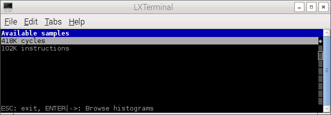
PERF first displays a screen that lists the event types for which profile data is available. In the following screenshot, data for two event types are available: cpu-cycles and instructions.
TUI responds to several keys as shown in the following table of key bindings.
  Navigation:
      h/?/F1                     Show this window
      UP/DOWN/PGUP/PGDN/SPACE    Navigate
      q/ESC/CTRL+C               Exit browser

  For multiple event sessions:

      TAB/UNTAB                  Switch events

  For symbolic views (--sort has sym):

      ->            Zoom into DSO/Threads & Annotate current symbol
      <-            Zoom out
      a             Annotate current symbol
      C             Collapse all callchains
      d             Zoom into current DSO
      E             Expand all callchains
      F             Toggle percentage of filtered entries
      H             Display column headers
      i             Show header information
      P             Print histograms to perf.hist.N
      r             Run available scripts
      s             Switch to another data file in PWD
      t             Zoom into current Thread
      V             Verbose (DSO names in callchains, etc)
      /             Filter symbol by name
UP, DOWN, right arrow, left arrow, etc. refer to navigation keys on a standard keyboard.
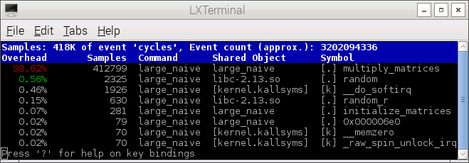
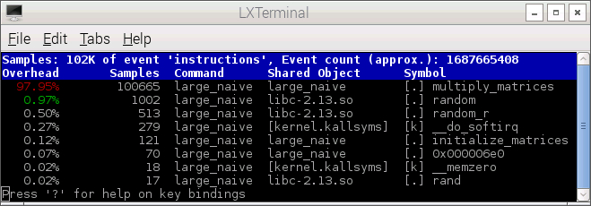
Use the UP and DOWN arrow keys to select the desired event and hit ENTER. PERF TUI displays a symbol-by-symbol distribution of samples for the selected event. The following two screenshots show the distribution of cpu-cycles event and instructions event samples.
Use the UP and DOWN arrow keys to select a symbol (e.g., the function multiply_matrices) and hit ENTER. PERF TUI displays a code-level profile, that is, the distribution of event samples across instructions and/or source code. The following screenshot shows the distribution of instructions event samples across the function multiply_matrices().
![]()
Here, PERF disassembles and displays the ARMv7 instructions that comprise the function multiply_matrices(). The function has three nested loops. I have drawn an arrow showing the innermost loop. As expected, the function spends most of its time in this loop and most of the retired instruction samples are attributed to code in the body of the innermost loop.
You probably noticed that the distribution of samples is "lumpy" even though all instructions within the loop body execute the same number of times. This is the effect of sampling skid. Skid is an artifact of the sampling process and is the result of several factors. PERF associates the performance event with the restart program counter (PC) address which it captures during interrupt handling. The restart PC rarely points at the instruction that actually caused the event and sampling interrupt. The restart PC address itself is subject to pipeline delays and other hardware conditions that affect interrupt detection, generation and dispatch. The net result is a lumpy distribution of event samples.
A statistically fair sampling process would produce a relatively even distribution of retired instruction event samples across the loop body. Precise attribution methods like IBS and PEBS eliminate skid. IBS, for example, produces an even distribution of retired op events for instructions that execute the same number of times.
Display event-based profiles: STDIO
In addition to TUI, PERF can print reports to Standard I/O through its STDIO interface. Just include the --stdio option on the command line:
perf report --stdio
The following command:
perf report -n --no-source --stdio --percent-limit 0.1
produces a symbol-by-symbol summary for each hardware performance event. (See the output below.) Of course, you may redirect the output to a file and save it. The --percent-limit option specifies a cut-off point for event statistics. Event percentages below the cut-off point are not displayed. Usually, these low percentage symbols (e.g., functions) are not significant factors in overall program performance and they can be ignored (suppressed).
# Samples: 418K of event 'cycles'
# Event count (approx.): 41856800000
#
# Overhead     Samples  Command      Shared Object      Symbol
# ........  ..........  ...........  .................  .....................
#
    98.62%      412799  large_naive  large_naive        [.] multiply_matrices
     0.56%        2325  large_naive  libc-2.13.so       [.] random
     0.46%        1926  large_naive  [kernel.kallsyms]  [k] __do_softirq
     0.15%         630  large_naive  libc-2.13.so       [.] random_r

# Samples: 102K of event 'instructions'
# Event count (approx.): 10277600000
#
# Overhead     Samples  Command      Shared Object      Symbol
# ........  ..........  ...........  .................  .....................
#
    97.95%      100665  large_naive  large_naive        [.] multiply_matrices
     0.97%        1002  large_naive  libc-2.13.so       [.] random
     0.50%         513  large_naive  libc-2.13.so       [.] random_r
     0.27%         279  large_naive  [kernel.kallsyms]  [k] __do_softirq
     0.12%         121  large_naive  large_naive        [.] initialize_matrices
As noted earlier, most of the cycles and instructions event samples are attributed to the function multiply_matrices().
The next step is to drill down into the hottest symbols, that is, the functions with the most event samples. These functions are the best candidates for tuning because they have the greatest impact on overall performance. The perf annotate command does this job for us:
perf annotate --stdio --dsos=large_naive --symbol=multiply_matrices --no-source
The command line above specifies the shared object (dsos) and specific symbol to be profiled. Here we drill down into the function multiply_matrices() inside of the shared object large_naive. This command produces the following text-only profile on the standard output.
 Percent |  Source code & Disassembly of large_naive for cycles
-------------------------------------------------------------------
         :
         :
         :
         :  Disassembly of section .text:
         :
         :  00008be0 :
    0.00 :  8be0:       push    {r4, r5, r6, r7, r8, r9, sl}
    0.00 :  8be4:       mov     r6, #0
    0.00 :  8be8:       ldr     sl, [pc, #124]  ; 8c6c
    0.00 :  8bec:       ldr     r4, [pc, #124]  ; 8c70
    0.00 :  8bf0:       ldr     r8, [pc, #124]  ; 8c74
    0.00 :  8bf4:       mov     r7, #4000       ; 0xfa0
    0.00 :  8bf8:       mul     r5, r7, r6
    0.00 :  8bfc:       mov     r0, #0
    0.00 :  8c00:       sub     r5, r5, #4
    0.00 :  8c04:       add     ip, r8, r5
    0.00 :  8c08:       add     r5, sl, r5
    0.06 :  8c0c:       vldr    s15, [pc, #84]  ; 8c68
    0.08 :  8c10:       mov     r1, r5
    0.00 :  8c14:       add     r2, r4, r0, lsl #2
    0.00 :  8c18:       mov     r3, #0
    2.75 :  8c1c:       add     r1, r1, #4
    2.71 :  8c20:       vldr    s14, [r2]
   82.77 :  8c24:       vldr    s13, [r1]
    3.67 :  8c28:       add     r3, r3, #1
    2.72 :  8c2c:       cmp     r3, #1000       ; 0x3e8
    0.00 :  8c30:       mov     r9, r1
    2.60 :  8c34:       vmla.f32        s15, s13, s14
    0.00 :  8c38:       add     r2, r2, #4000   ; 0xfa0
    2.60 :  8c3c:       bne     8c1c
    0.02 :  8c40:       vmov    r3, s15
    0.00 :  8c44:       add     r0, r0, #1
    0.00 :  8c48:       cmp     r0, #1000       ; 0x3e8
    0.00 :  8c4c:       str     r3, [ip, #4]!
    0.00 :  8c50:       bne     8c0c
    0.00 :  8c54:       add     r6, r6, #1
    0.00 :  8c58:       cmp     r6, #1000       ; 0x3e8
    0.00 :  8c5c:       bne     8bf8
    0.00 :  8c60:       pop     {r4, r5, r6, r7, r8, r9, sl}
    0.00 :  8c64:       bx      lr
    0.00 :  8c68:       .word   0x00000000
    0.00 :  8c6c:       .word   0x007b43e8
    0.00 :  8c70:       .word   0x003e3ae8
    0.00 :  8c74:       .word   0x000131e8
This profile shows the distribution of cycles event samples in the function multiply_matrices(). The hot inner loop consists of the nine instructions starting at address 0x8c1c and ending at address 0x8c3c. The distribution across the inner loop is not numerically even due to sampling skid.
Because sampling is a statistical process, we need to determine how much confidence to assign to results within a function or code region. From statistics theory, we know that confidence increases with sample size, i.e., confidence is higher when more samples are taken from a population. As a rough rule of thumb, I wouldn't put too much confidence into a localized profile unless there are at least 100 samples per instruction in the code region of interest. In the profile above, nearly all of the 412,799 cycles event samples attributed to multiply_matrices() are within the innermost loop. Thus, our confidence in the profile is very high and any inferences that we draw about loop behavior should be valid.
Display useful run information
PERF saves meta-information about the data collection process in the perf.data file. This is quite handy because it's easy to get confused when comparing a large number of runs during analysis, e.g., "What events did I collect? What was the sampling period?"
The following command:
perf evlist
displays the performance event types captured in perf.data. Add the -F command line option to display the sampling period (or frequency) as shown here:
perf evlist -F
PERF displays the event types and sampling periods:
cycles: sample_freq=100000
instructions: sample_freq=100000
Sometimes you need more detailed information about a run, including characteristics of the underlying software and hardware platform. The command:
perf report --header-only
displays a summary of the platform characteristics, the perf record command that was used to collect data, and the internal PERF configuration for each event.
# ========
# captured on: Wed Mar 25 14:40:56 2015
# hostname : raspberrypi
# os release : 3.18.9-v7+
# perf version : 3.18.5
# arch : armv7l
# nrcpus online : 4
# nrcpus avail : 4
# cpudesc : ARMv7 Processor rev 5 (v7l)
# total memory : 949424 kB
# cmdline:/usr/bin/perf_3.18 record -c 100000 -e cycles,instructions ./large_naive
# event : name = cycles, type = 0, config = 0x0, config1 = 0x0, config2 = 0x0,
    excl_usr = 0, excl_kern = 0, excl_host = 0, excl_guest = 1, precise_ip = 0,
    attr_mmap2 = 1, attr_mmap  = 1, attr_mmap_data = 0, id = { 28, 29, 30, 31 }
# event : name = instructions, type = 0, config = 0x1, config1 = 0x0,
    config2 = 0x0, excl_usr = 0, excl_kern = 0, excl_host = 0, excl_guest = 1,
    precise_ip = 0, attr_mmap2 = 0, attr_mmap  = 0, attr_mmap_data = 0,
    id = { 32, 33, 34, 35 }
# HEADER_CPU_TOPOLOGY info available, use -I to display
# pmu mappings: software = 1, tracepoint = 2, armv7_cortex_a7 = 4, breakpoint=5
# ========
#
Comparative analysis
I ran large_naive and large_interchange, and collected event sample data for the most relevant hardware events. A comparative summary is shown in the following table.
| Metric | large_naive | large_interchange |
|---|---|---|
| Elapsed time | 45.25 seconds | 20.17 seconds |
| instructions | 94,553 samples | 93,969 samples |
| cycles | 406,284 samples | 184,310 samples |
| cache-references | 20,995 samples | 31,020 samples |
| cache-misses | 9,960 samples | 734 samples |
| LLC-loads | 19,839 samples | 1,458 samples |
| LLC-load-misses | 699 samples | 654 samples |
| dTLB-load-misses | 9,324 samples | 29 samples |
| branches | 10,234 samples | 10,268 samples |
| branch-misses | 81 samples | 54 samples |
We can see a sharp reduction (from large_naive to large_interchange) in cycles, cache-misses, LLC-loads and dTLB-load-misses. Elapsed time is cut in half. You should compare this table against the corresponding measurements made by PERF event counting mode. The number of samples for each event is roughly equal to 1/100,000 times the number of individual events as measured by counting mode. This is consistent with a sampling period of 100,000 because each event sample is worth 100,000 individual events of the same event type.
I also calculated the key rates and ratios from the event sample counts as shown in the following table. The rates and ratios are consistent with the values computed with the raw event counts measured by PERF counting mode. (Please see the corresponding table near the beginning of this article.)
| Ratio or rate | large_naive | large_interchange |
|---|---|---|
| IPC | 0.23 | 0.51 |
| Cache miss ratio | 0.47 | 0.02 |
| Cache miss rate PTI | 105.33 | 7.81 |
| LLC load miss ratio | 0.03 | 0.45 |
| LLC load miss rate PTI | 7.39 | 6.96 |
| dTLB load miss rate PTI | 98.61 | 0.31 |
| Branch mispredict ratio | 0.01 | 0.01 |
| Branch mispred rate PTI | 0.86 | 0.57 |
The cache miss rate per thousand instructions (PTI) and dTLB load miss rate PTI are much lower for large_interchange. The loop nest interchange algorithm has a more efficient and penalty-free memory access pattern. IPC is cut in half.
Overhead
Let's calculate the sampling overhead for both large_naive and large_intersection. We subtract the baseline (no sampling) elapsed time from the largest elapsed time with sampling enabled, then divide by the baseline time. The overhead for large_naive is:
(45.25 - 42.72) / 42.72 = 2.53 / 42.72 = 5.92%
The sampling overhead for large_intersection is:
(20.17 - 19.39) / 19.39 = 0.78 / 19.39 = 4.02%
Thus, the actual sampling overhead is close to our 5% target in both cases when the fixed sampling period is 100,000.
Copyright © 2015 Paul J. Drongowski