Raspberry Pi 4 ARM Cortex-A72 processor

Raspberry Pi 4 (RPi4) is a big step beyond the earlier models 1, 2 and 3. Both desktop interaction and browsing are snappier and don’t have that laggy feel. I haven’t even thought (yet) about the RPi4’s music making and synthesis potential!

The Raspbeery Pi 4 is powered by a new processor from Broadcom: the BCM2711. The BCM2711 is an improvement over the BCM2835/2836 used in earlier models. Like the BCM2836, main memory is external. I’m running an RPi with 4GB of RAM (LPDDR4-3200 SDRAM, 3200Mb/s, dual channel). The old RPi2 has only 1GB of RAM. The BCM2711 supports Gigabit Ethernet (1000 BaseT) while the old RPi2 is just 100Megabit Ethernet. Faster Internet speed makes updates and browsing so much faster.

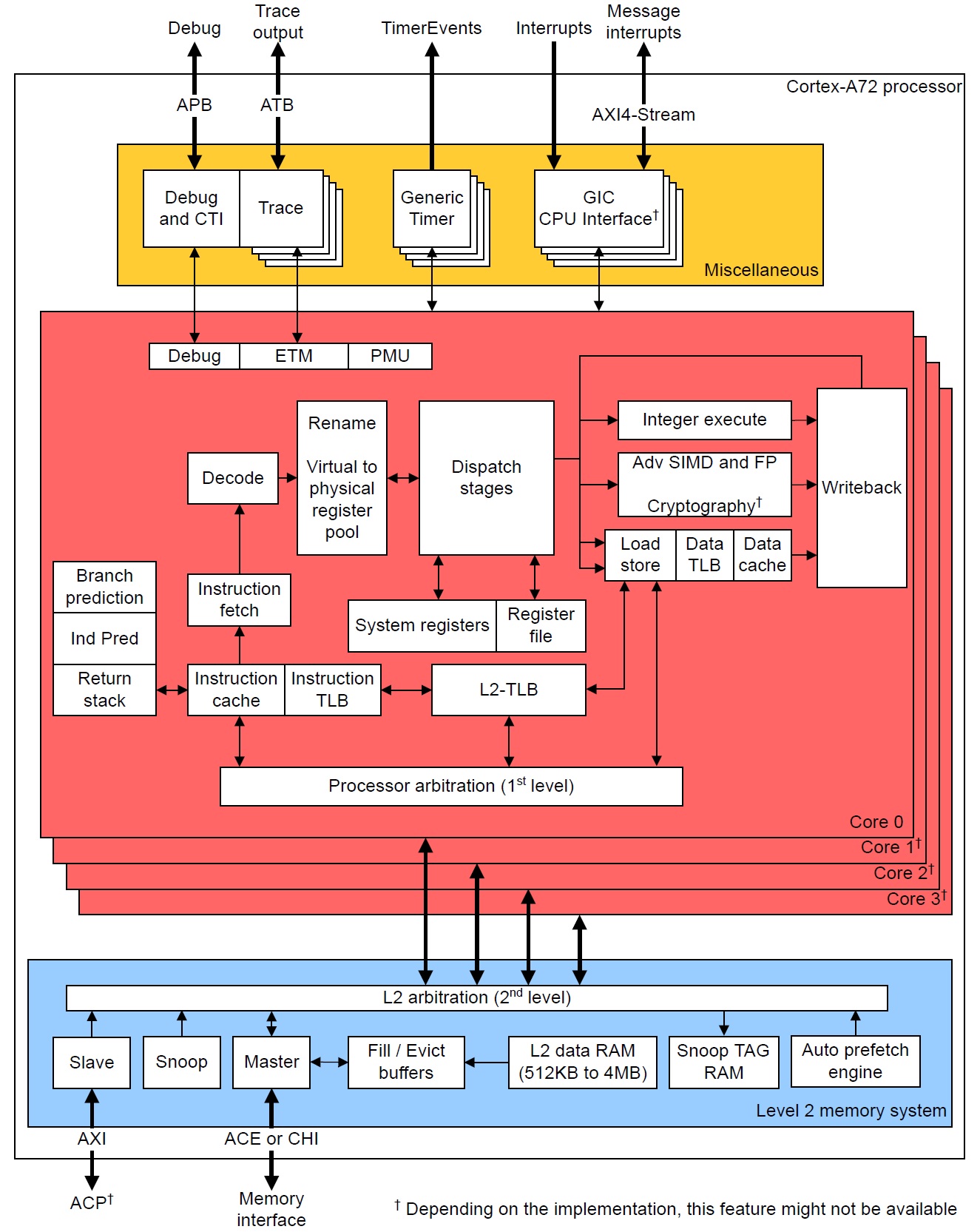
The RPi4 is a quad-core ARM Cortex-A72 processor clocking at 1.5GHz. The old RPi2 is a 900MHz quad-core ARM Cortex-A7 processor. The old BCM2835 is a member of the ARM11 family (ARM1176JZF-S, to be exact). The ARM Cortex-A72 within the BCM2711 has a much improved CPU core and memory subsystem.

The old ARM1176 is a relatively simple beast. It is a single issue machine, that is, it issues a single instruction per cycle. The ARM1176 core has eight pipeline stages and three execution pipes: 1. ALU, shift, saturation, 2. Multiply-accumulate, and 3. Load/store.

The Cortex-A72, on the other hand, performs 3-way instruction decoding and can issue as many as five operations per cycle. It is an out-of-order superscalar machine allowing speculative issue. That is waaay more sophisticated than the ARM1176, putting the Cortex-A72 on the same level as x86 superscalar machines. In fact, it translates ARM instructions into micro-ops like most modern x86 superscalar processors. It even performs micro-op fusion in some cases. The Cortex-A72 performs register renaming, letting micro-ops (instructions) execute when program data are ready (out-of-order execution, in-order retirement).

The Cortex-A72 issues micro-ops to eight execution pipelines:

  • Branch: Branch micro-ops
  • Integer 0: Integer ALU micro-ops
  • Integer 1: Integer ALU micro-ops
  • Integer Multi-Cycle: Integer shift-ALU, multiply, divide, CRC and sum-of-absolute differences micro-ops
  • FP/ASIMD 0: ASIMD ALU, ASIMD misc, ASIMD integer multiply, FP convert, FP misc, FP add, FP multiply, FP divide and crypto micro-ops
  • FP/ASIMD 1: ASIMD ALU, ASIMD misc, FP misc, FP add, FP multiply, FP square root and ASIMD shift micro-ops
  • Load: Load and register transfer micro-ops
  • Store: Store and special memory micro-ops

Up to 5-way issue and a larger number of independent execution pipelines permit more fine-grained parallelism than ARM1176. Of course, the compiler must know how to exploit all of this parallelism, but the potential is there. The ARM Cortex-A72 Software Optimization Guide specifies the number of execution cycles and pipeline units for each kind of ARM instruction. This information is incorporated into a compiler and guides the choice and scheduling of machine instructions.

ARM Cortex-A72 block diagram

The Cortex-A72 allows speculative execution. Without speculation, a CPU must wait at each conditional program branch until the direction is decided and instruction fetch can proceed along the chosen branch. The Core-A72 processor predicts branch direction (speculates) and aggressively issues instructions along predicted branches. The Cortex-A72 branch predictor is also improved over ARM1176. (I’m still digging into details.) If a branch is mispredicted, speculative results are discarded. So, it’s important to have a good branch predictor.

The Cortex-A72 can perform a load operation and a store operation every cycle because it has separate load and store pipelines. The ARMv8-A instruction set architecture (ISA) allows arbitrary data alignment and access. However, the Cortex-A72 hardware penalizes load operations that cross a cache-line (64-byte) boundary and store operations that cross a 16-byte boundary. Programmers (and compilers) should keep that in mind when laying down data structures in memory.

Like all modern high-performance computers, the Cortex-A72 organizes physical memory into a hierarchy with the fastest/smallest memory (registers) near the arithmetic/logic unit (ALU) and the slowest/largest memory (RAM) far away and off-chip. The registers and RAM are connected to intervening levels of memory — the caches:

          Register          Fast, but small 
|
Level 1 caches
|
Level 2 cache
|
RAM Big, but slow

Data and instructions are read (and written) in efficient chunks making data and instructions available when needed by the registers and ALU. The chunks are called “cache lines.” Thanks to cache memory, programs run faster when they (re)use data that are close together in memory (i.e., occupy the same cache line) and are the most recently accessed. These notions are called “spatial locality” and “temporal locality.”

The following table is a quick summary of the level 1 and level 2 cache structures of the ARM1176 and Cortex-A72.

Feature ARM1176 Cortex-A72
L1 I-cache capacity 16KB 48KB
L1 I-cache organization 4-way set associative, 32B line 3-way set associative, 64B line
L1 D-cache capacity 16KB 32KB
L1 D-cache organization 4-way set associative, 32B line 2-way set associative, 64B line
L2 cache capacity 128KB 1MB
L2 cache organization Shared, 8-way set associative, 64B line Shared, 16-way set associative, 64B line

Each core has an Instruction Cache (I-Cache) and Data Cache (D-Cache). The four cores share the Level 2 (L2) cache.

As you can see, the RPi4 (BCM2711) has larger caches and a bigger cache line size (64 bytes) than ARM11. RPi4 programs are more likely to find instructions and data in cache than earlier RPi models.

Contemporary processors have one or more memory management units (MMU) that break physical RAM into logical pages. This scheme is called “virtual memory.” The MMU translate logical program addresses (from loads, stores and instruction fetches) into physical RAM addresses. Address translation has its own memory hierarchy:

   Translation registers       Fast, but only a single mapping 
|
Level 1 TLBs
|
Level 2 TLB
|
RAM Big page tables, but slow

Page tables in RAM are maps that describe the layout of pages in the operating system and application programs. Translation lookaside buffers (TLB) are cache-like hardware structures that hold the most recently used (MRU) address translation information, i.e., where a logical page is located in physical memory. TLBs greatly speed up the translation process by keeping MRU page table information on-chip within the CPU.

Cortex-A72 has larger translation lookaside buffers (TLB) than ARM1176, as summarized in the table below. With larger TLBs, a program can touch more locations in memory without triggering a performance robbing page fault — an event which brings page translation information into the CPU from relatively slow RAM.

Feature ARM1176 Cortex-A72
D-MicroTLB capacity 10 entries 32 entries
D-MicroTLB organization Fully assoc, 1 lookup/cycle Fully assoc, 1 lookup/cycle
I-MicroTLB capacity 10 entries 48 entries
I-MicroTLB organization Fully assoc, 1 lookup/cycle Fully assoc, 1 lookup/cycle
L2 TLB capacity 256 entries 1024 entries
L2 TLB organization Unified, 2-way set assoc Unified, 4-way set assoc

Each core has a Data Micro-TLB (D-MicroTLB), Instruction Micro-TLB (I-MicroTLB), and Level 2 (L2) TLB. (In ARM1176 terminology, the L2 TLB is called the “Main TLB”).

In summary, the RPi4’s BCM2711 processor is a powerhouse even though it won’t knock that gaming machine off your desktop. 🙂 If you’ve been waiting to dive into Raspberry Pi or to upgrade, please don’t hesitate any longer.

I’m getting the itch to play with RPi4’s hardware performance counters and post results. In the meantime, check out my summary of the ARM11 micro-architecture. If you would like to know more about performance measurement and events in ARM1176-based Raspberry Pi’s, please see my Performance Events for Linux (PERF) tutorial.

Also, I have uploaded all of my teaching notes about computer design, VLSI systems and computer architecture:

These resources should help students and teachers alike!

Copyright © 2020 Paul J. Drongowski

Memory access time

In my last post, I used a simple pointer chasing loop to characterize the different levels of the BCM2835 (Raspberyy Pi) memory hierarchy. I ran the pointer chasing loop for a range of linked list sizes where the list size determines the storage level to be exercised. For example, a linked list occupying 16KB or less causes the chase loop to exercise the level 1 (L1) data cache. I measured hardware performance events for each test case and summarized the results in a table. The results clearly show three different timing tiers: L1 data cache, access to primary memory (no TLB miss) and access to primary memory with a Main TLB miss. A miss in the Main TLB is quite slow because the hardware page table walker must read page mapping information from primary memory in order to update the TLB and to complete the memory operation in flight.

The one characteristic missing from the analysis, however, is the estimated access time for each level. Sure, the execution times clearly break the test cases into tiers, but elapsed execution time does not really measure the access (latency) time itself.

In the next experiment, I estimate the access time. (See the source code in latency.c.) The approach is essentially unchanged from the first experiment: use pointer chasing on lists of different sizes to hit in particular levels of the memory hierarchy. Like the first experiment, the program (named latency) successively traverses the same linked list many times (default: 1000 traversals). Part way through each traversal, the loop chooses a chase operation and measures its execution time. The sampled execution time is saved temporarily in an array until all traversals are complete. Then, the program writes the execution times to a file named samples.dat. The samples are aggregated into a histogram which shows the distribution of the times.

The sampling technique lets each full traversal get underway before taking a measurement in order to “warm up” the pipeline, cache and TLBs. Taking a single sample per traversal avoids major cache and TLB pollution due to the bookkeeping needed to take and save samples. The measured execution times should faithfully represent access time (plus some measurement bias).

The program measures execution time in cycles. It configures and enables the ARM1176 Cycles Counter Register (CCR) as a free-running cycles counter. The program resets and enables the CCR before starting a traversal, thus avoiding a counter overflow. (A full traversal completes before the CCR overflows.) The pointer chasing loop reads the CCR before chasing the next pointer and reads the CCR after chasing the pointer. The difference between the after and before counts is the estimated execution time of the chase operation. The chase operation is implemented as a single ARM load instruction, so the instruction execution time is a biased estimate of the memory access time.

Here is the code for the function sample_cycles() and the pointer chasing loop within. The function takes two arguments: a pointer to the head of the linked list and an integer value that chooses the chase operation to be sampled.

uint32_t sample_cycles(CacheLine* linked_list, int n)
{
  register CacheLine* item ;
  register uint32_t before, after, cycles ;
  register count = n ;

  cycles = 0 ;
  for(item = linked_list ; item != NULL ; ) {
    if (count-- == 0) {
      before = armv6_read_ccr() ;
      item = item->ptrCacheLine[0] ;
      after = armv6_read_ccr() ;
      cycles = after - before ;
    } else {
      item = item->ptrCacheLine[0] ;
    }
  }

  return( cycles ) ;
}

On each iteration, the loop body checks and decrements the sampling count maintained in the variable count. If the sampling count is not zero, then the loop quickly performs an ordinary chase operation. If the count is zero, then the code snaps the before and after CCR values by calling armv6_read_ccr(), an in-line function that performs an ARM MRC instruction to read CCR. The difference is computed and is saved in the variable cycles until it can be returned by the function after traversal. The chase loop exits when it reaches the NULL pointer at the end of the linked list.

Local variables are allocated to general registers in order to avoid extraneous cache and TLB references that would perturb measurements. I checked the compiled machine code to make sure that the compiler accepted the register hints and actually allocated the local variables to registers. I also made sure that the function armv6_read_ccr() was expanded in-line.

The latency program needs to have user-space access to the ARM1176 performance counters. You must load the aprofile kernel module before running latency. Otherwise, you will get an “Illegal instruction” exception when the program attempts to configure the performance counters.

Here is a histogram showing the distribution of execution time samples when the linked list is 8KB in size. The 8KB test case consistently hits in the L1 data cache.

9  1000 ################################################

The first column is the execution time in cycles. The second column is the number of samples with the value shown in the first column. All 1,000 samples are 9 cycles.

Chapter 16 of the ARM1176JZF-S Technical Reference Manual (TRM) describes instruction cycle timings. A load from L1 data cache has a 3 cycle load-to-use latency (access) time. Taking 3 cycles as the actual access time, I estimate a measurement bias of (9 cycles – 3 cycles) = 6 cycles due to the pipelined execution of the ARM MRC instructions that read the CCR and the load instruction that chases the linked list pointer.

The 32KB and 64KB test cases form the middle timing tier. Both test cases are within the coverage of the Main TLB (288KB) and memory accesses hit in either the Micro TLB or Main TLB. The distributions are similar. Here is the distribution for the 64KB case.

 9   49 ##### 
17    1 # 
61  320 ##########################
62  571 ################################################
63   11 # 
64    4 # 
65    1 # 
69    1 # 
70   27 ### 

There is a strong peak in the narrow range of [61:62] cycles. The nonbiased estimate for access time to primary memory with a TLB hit is (62 cycles – 6 cycles bias) = 56 cycles.

The test cases at 256KB and larger form the third timing tier. These cases exceed the Main TLB coverage. (The 256KB case almost occupies the entire Main TLB and the performance event data place this case in the third and longest running tier.) Load operations miss in the Main TLB forcing a hardware page table walk. The table walker performs at least one additional primary memory read operation in order to obtain page mapping information for the TLB. Here is the distribution for the 1MB case.

113    4 # 
116  224 ##############################################
117   23 ###### 
118   59 ############## 
119  129 ###########################
120    5 ## 
121  224 ##############################################
122  185 ############
125    4 # 
130    9 ### 
132    7 ## 
133   18 ##### 
135    5 ## 

The samples are clustered in the range of [116:122] cycles. The nonbiased estimate for access time to primary memory with a Main TLB miss is (122 cycles – 6 cycles bias) = 116 cycles. This is approximately twice the access time of a load that hits in either the data MicroTLB or the Main TLB.

The following table summarizes the access time for each level of the memory hierarchy.

Level Access time Condition
CPU register 1 cycle
L1 data cache 3 cycles Data cache hit
Primary memory 56 cycles No TLB miss
Primary memory 116 cycles Main TLB miss
Memory hierarchy access times (latencies)

Where is the L2 cache? The BCM2835 dedicates the L2 cache to the Broadcom VideoCore GPU. Memory operations from the CPU are routed around the L2 cache. The L2 cache is not a factor here and is not part of the analysis.

From these estimates, we can see why the textbook (naive) matrix multiplication program is so slow. The textbook algorithm does not walk sequentially through one of its operand arrays. The long memory stride causes a large number of Main TLB misses. Memory access is twice as slow when an access misses in the Main TLB, thereby slowing down program execution and increasing elapsed time.

Performance events and Zen

It’s always interesting to get started with a new microarchitecture and the ARM 1176 inside of the Raspberry Pi is no exception.

Back when we were in school, we all dutifully went to computer architecture class and learned about memory hierarchy, read/write access, cache memory, and the translation lookaside buffer (TLB). A hit was a clean hit and a miss was, well, a miss.

Real world behavior of cache memory and the TLB is far more complicated. Computer designers study the behavior of benchmark and application programs in order to find behavioral patterns which the hardware can exploit for speed. This includes behavior like sequential access, fixed-length address strides, temporal and spatial locality. Then the designers build hardware which implements every trick in the book, all in the name of faster access to memory data and ultimately, faster programs. In the case of low-power machines like ARM, computer designers use behavioral patterns to turn off or not actively use functional components in order to save power. Inactive components don’t consume power, but they don’t generate observable signals either.

A real world performance event is a dynamic condition which occurs in the midst of this complicated hardware. An access or miss may be counted only for the first of multiple sequential reads/writes to the same cache line. Other undocumented internal microarchitectural conditions affect the event counts. Suddenly, it’s not so easy to interpret performance event counts armed with our textbook notions of cache access and cache miss. It may not even be possible to effectively compare the behavior of two versions of the same program (one version tuned, the other version untuned).

We can whine, whinge and kvetch about the limitations of real world performance events, the lack of documentation, and other shortcomings. At the end of the day, the performance events are what they are and we need to accept them. Therein lies the Zen of performance events.

The fine print in the TRM

I’ve been busy writing up the first example showing how to use the Raspberry Pi performance counter kernel module and the ARM11 performance counters. These write-ups always take longer than I think, so here’s a few small things that I’ve learned along the way.

Run, don’t walk, to the ARM web site and download a copy of the ARM1176JZF-S Technical Reference Manual. The TRM has the goodies and details about the ARM1176 core in the Raspberry Pi. This includes information about cache and TLB sizes, branch prediction, instruction timing and, of course, the performance counters and events. The TRM is essential reading if you want to know more about the processor at the heart of the Raspberry Pi.

Good as it is, the TRM doesn’t contain all of the information and in some cases, the descriptions are very low level and esoteric. Computer designers describe hardware from their point of view, which is not necessarily the perspective of a software engineer. In fact, the terminology is often quite foreign to the ears of a software engineer. The TRM is no exception.

The first question many people ask about the Raspberry Pi is “What happened to the L2 cache?” The L2 cache is not part of the ARM1176 core, so the TRM describes the interface to the L2 and is mum about the L2 itself. The best clues about the L2 cache appear at the beginning of the Broadcom BCM2835 ARM Peripherals manual. Broadcom has implemented a pretty decent graphics processing unit (the VideoCore) and are reluctant to release too many details about it lest competitors learn too much about their design. The diagram at the beginning of the peripherals manual shows the memory layout and bus structure of the BCM2835. There are actually two memory management units (MMU). The ARM MMU maps program virtual addresses to physical addresses and the VC/ARM MMU maps physical addresses onto the VC/CPU bus and real honest to goodness physical memory. The high order bits of the VC/CPU address determine the cacheable status of memory regions including, TA-DA!, the L2 cache. The footnote on page 6 says, “BCM2835 provides a 128KB system L2 cache, which is used primarily by the GPU. Accesses to memory are routed either via or around the L2 cache depending on senior two bits of the bus address.” So, under normal circumstances, memory reads/writes made by a program are not routed through the L2 cache. I suspect, and this is a guess, that the L2 cache boosts the bandwidth for the memory hungry GPU. Well, we may never really know.

The ARM1176 has two separate level 1 (L1) caches: a 16KB instruction cache and a 16KB data cache. I verified the cache size using the coprocessor’s Cache Type Register. The TRM is not always clear about the number and size of the translation lookaside buffers (TLB). There are two level 1 MicroTLBs. Each MicroTLB has ten entries. The MicroTLBs are backed by a Main TLB consisting of eight fully associative elements and a 64 element low-associativity store. Depending on how Linux uses the eight fully associative, lockable entries, as many as 72 entries are available for address translation.

The other characteristics that require some digging are the load-to-use latencies for the L1 cache and the TLBs. I’m just diving into the instruction timing information in Chapter 16 of the TRM. However, the load-to-use latency for a hit in the L1 data cache is three cycles. That is, the data from a load hitting in the L1 data cache is not available for 3 cycles once the load is issued. Dedicated datapaths called bypasses forward load data to other instructions in the pipeline.

The Load/Store Unit does not always block on an L1 data cache miss and supports hit under miss (HUM). The miss goes into a holding state/buffer and non-dependent instructions are allowed to execute. Up to three outstanding misses are allowed. This increases parallelism letting some computations proceed even when a load misses in the L1 data cache.

Finally, the ARM1176 is a single issue machine, that is, one instruction is issued at a time. This constraint simplifies the issue logic. The ARM1176 doesn’t need to implement any complicated issue rules to determine whether two or more instructions of a certain type can issue in the same cycle. Instructions are issued in-order, but out-of-order completion is allowed. out-of-order completion increases exploitable fine-grained parallelism.

Another neat feature of the ARM — nearly all instructions can be predicated. An enabling condition (a predicate) can be defined for an instruction. The enabling condition gates the execution of the instruction. Predication is cool and is used to eliminate branches. More about predication one of these days…

Hope you enjoyed this trip through the fine print!

Performance counter kernel module

As promised, I’ve described the design of a Linux loadable kernel module that allows user-space access to the Raspberry Pi (ARM 1176) performance counters. By the way, the design of the module is not specific to Raspbian Wheezy or even the Raspberry Pi for that matter. I believe that the kernel module could be used on the new Beagleboard Black (BBB) to enable user-space counter access on its ARM Cortex-A8 processor under Linux. I just ordered a BBB and will try out the code when possible. (Assuming quick delivery!)

The kernel module alone isn’t enough to measure performance events. In fact, the kernel module doesn’t even touch the counters. It merely flips a privileged hardware bit which lets user-space programs read and write the performance counters and control register. So, I have also written a few user-space C functions to configure, clear, start and stop the performance counters. An application program just needs to call a few functions to choose the events to be measured and start counting, to stop counting, to get the raw counts, and to print the event counts.

I have uploaded the source for both the kernel module (aprof.c) and the user-space functions (rpi_pmu.h and rpi_pmu.c). In addition, there is source for some utility functions that I like to use in benchmark programs (test_common.h and test_common.c). All of this is a work in progress and I will update the source when major enhancements or changes are made.

Speaking of source, I have found a way of organizing and storing source code through WordPress. WordPress is kind of security paranoid and doesn’t allow you to upload source code or even gzip’ed TAR files. I ran into this issue when I attempted to upload a make file and WordPress wouldn’t let me do it (with complaints about potentially malicious code and so forth). WordPress does let you post source for viewing, however.

So, I’ve added a Source menu item to the main menu. I want the menu structure below the Source item to operate like a browsable code repository. The first level of items below Source are projects, like the kernel module. The next level of menu items navigate into the source belonging to a project. Each make file and source file is a separate page. The source code is displayed using the SyntaxHighligher plug-in in order to keep indentation. No other formatting or highlighting is done just to keep things simple. I could cut and paste code from these pages, so I hope you can, too!

An introduction to performance tuning (and counters)

My latest page is an overview of performance tuning on ARM11. The Raspberry Pi is a nifty little Linux box, but it’s kind of slow at 700MHz. Therefore, I suspect that programmers will have an interest in tuning up application programs and making them run faster. Performance tuning is also a good opportunity to learn more about computer architecture and machine organization, especially the ARM1176 core at the heart of the Raspberry Pi and its memory subsystem.

The ARM1176 has three performance counters which can measure over 20 different microarchitectural events. One of these counters is dedicated to core clock cycles while the other two are configurable. The new performance tuning page has a brief overview of the counters and it has a table with the supported events.

The new page also describes two different use cases for the counters: caliper mode and sampling mode. Caliper mode counts the number of microarchitectural hardware events that occur between two different points in program execution. Caliper mode is good for measuring the number of data cache accesses and misses for a hot code region like a loop. The programmer inserts code to start counting at the beginning of the hot region and inserts code to stop counting at the end of the hot region. This is the easiest use case to visualize and to implement. It’s the approach that I’m taking with my first performance measurement software and experiments (a custom kernel module plus some user-space code). These experiments are almost finished and ready for write up.

Sampling is a statistical technique that produces an event profile. A profile shows the distribution of events across program instructions, routines, source lines, or modules. This is a good way to find hot-spots in a program where tuning is most beneficial. Sampling does not require modification to source.

Performance Events for Linux (informally called “PERF”) is the standard tool for program profiling on Linux. At the moment, PERF has a bug which prevents it from sampling hardware events. I’ve been looking into this problem, too, and hope to post some results. In the long-run, I want to post examples using PERF in order to help people tune up their programs on Raspberry Pi.