Given the scarcity of combo organ top octave generator ICs, what’s a hack supposed to do? Emulate!
I posed a “bar bet” against myself — can I emulate a top octave generator chip with an Arduino? The Arduino is a bit slow and I wasn’t sure if it would be fast enough for the task. Good thing I didn’t best against it…
If you browse the Web, you’ll find other solutions. I chose Arduino UNO out of laziness — the IDE is already set-up on my PC and the hardware and software are easy to use. Plus, I have UNOs to spare. Ultimately, one can always cobble together a barebones solution consisting of an ATMEGA328P, a 16MHz crystal and a few discrete components, if small size is an issue.
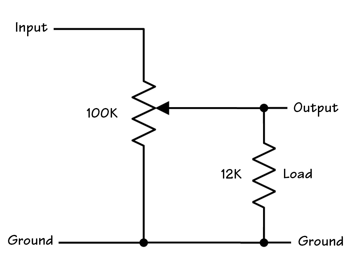
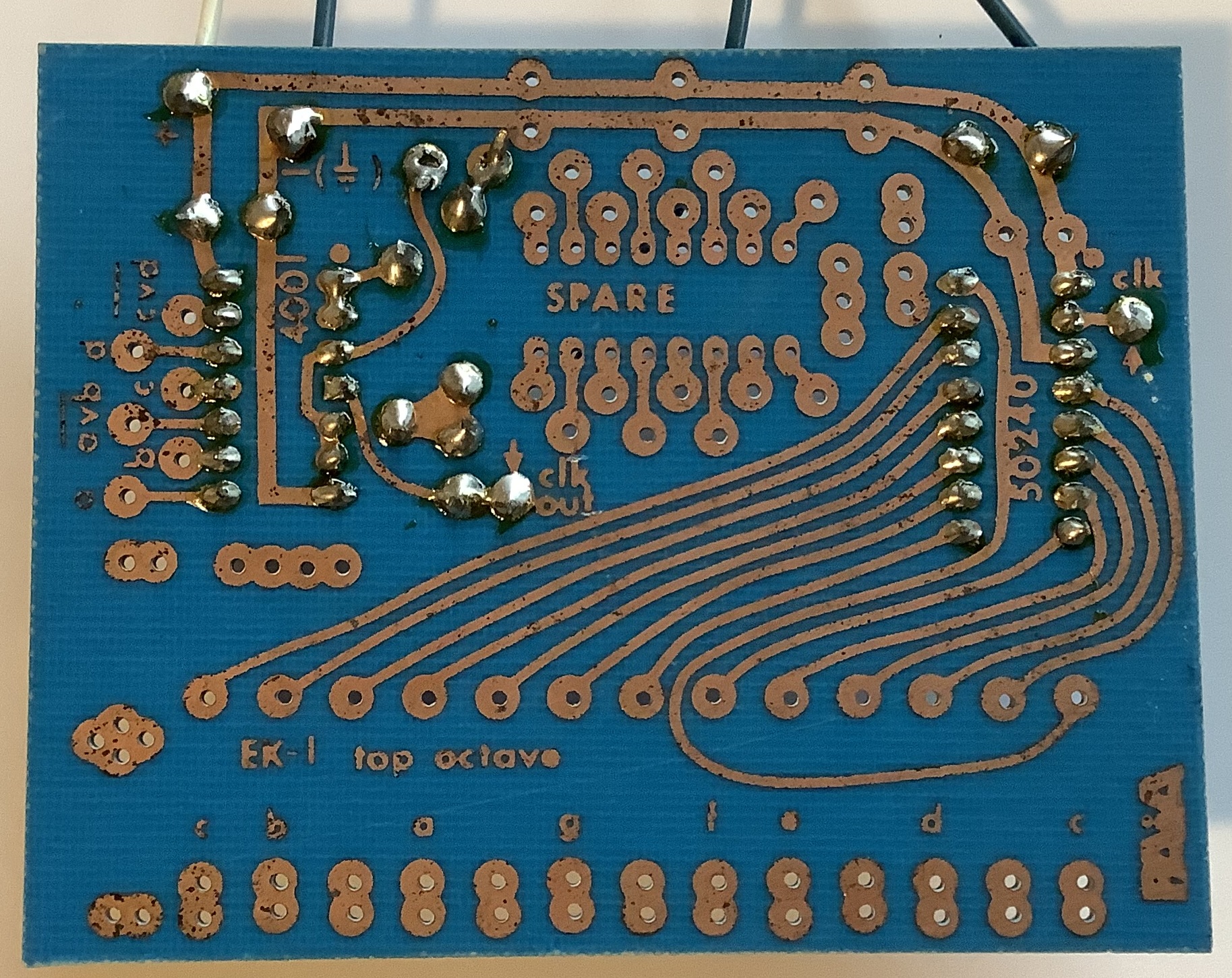
There’s not much ancilliary hardware required. A few jumper wires bring out ground and audio signals from the UNO. I passed the audio through a trim pot volume circuit in order to knock the 5 Volt signal down to something more acceptable for a line level input. The trim pot feeds a Sparkfun 3.5mm phone break-out board which is connected to the LINE IN of a powered speaker.
That’s it for the test rig. The rest is software.
I assigned a “root” pitch to Arduino digital pins D2 to D13:
#define CnatPin 13
#define BnatPin 12
#define AshpPin 11
#define AnatPin 10
#define GshpPin 9
#define GnatPin 8
#define FshpPin 7
#define FnatPin 6
#define EnatPin 5
#define DshpPin 4
#define DnatPin 3
#define CshpPin 2
Thankfully, the Arduino has just enough available pins to do the job while avoiding pins D1 and D0. D1 (TX) and D0 (RX) carry the serial port signals and it’s best to let them do that job alone.
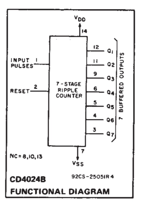
My basic thought algorithm-wise was to implement 12 divide-down counters (one per root pitch) that decrement during each trip through a non-terminating loop. Each counter is (pre-)loaded with the unique divisor which produces its assigned root pitch. Whenever a counter hits zero, the code flips the corresponding digital output pin. If the loop is fast enough, we should hear an audio frequency square wave at the corresponding digital output. This approach is (probably) similar to the actual guts of the Mostek MK50240 top octave generator chip, except that the MK50240 counters operate in parallel.
Each root pitch needs:
- A digital output pin
- A note count variable
- A divisor
- A state variable to remember if the output is currently 0 or 1
For the highest pitch, C natural, we need declarations:
    #define CnatPin 13

    byte CnatCount ;

    #define CNAT (123)

    byte CnatState ;
and count down code to be placed within the loop body:
    if (--CnatCount == 0) {
      digitalWrite(CnatPin, (CnatState ^= 0x01)) ;
      CnatCount = CNAT ;
    }
These are the basic elements of the solution. The rest of the pitches follow the same pattern.
Now, for the fun — making the loop fast enough to be practical. This was a bit of a journey!
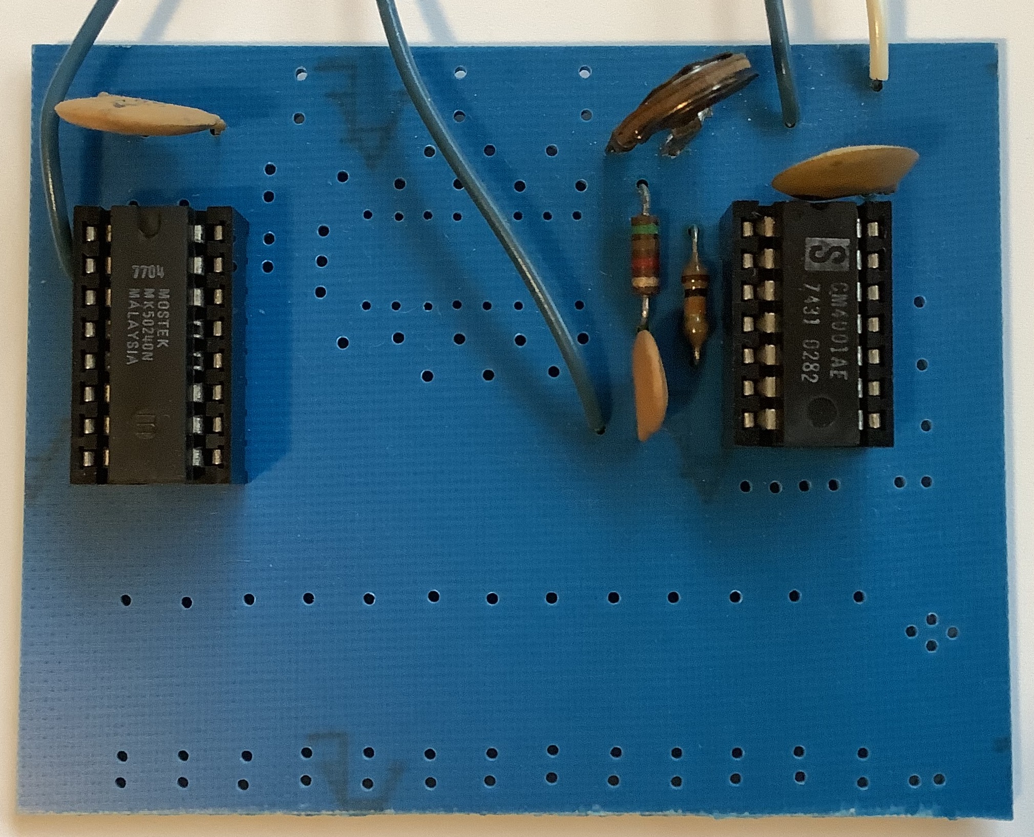
First off, I tried the MK50240 divisor values which require at least 9 bits for representation. Using INT (16-bit) counter variables, everything worked, but the final note frequencies were too low — not much “top” in top octave. I cut the divisor values in two, switched to BYTE (8-bit) counter variables, and doubled the output frequencies. Yes, AVR (Arduino) BYTE arithmetic is roughly twice as fast as INT arithmetic. That was the first lesson learned.
The next lesson had to do with how the counters were stored (register vs. memory). If I were writing the code in assembler language, I would have stored all of the counters in AVR CPU registers. (AVR has 32 CPU registers, after all.) Register storage would provide the fastest counter access and arithmetic. However, this is where C language and the Arduino setup()/loop() structure fight us.
Ultimately, I put all code into setup() and ditched loop(). I declared all twelve counters as register BYTE variables in setup():
    register byte CnatCount ;
    register byte BnatCount ;
    register byte AshpCount ;
    register byte AnatCount ;
    register byte GshpCount ;
    register byte GnatCount ;
    register byte FshpCount ;
    register byte FnatCount ;
    register byte EnatCount ;
    register byte DshpCount ;
    register byte DnatCount ;
    register byte CshpCount ;
The compiler allocated the counter variables to AVR CPU registers. This enhancement doubled the output frequencies, again. Now we’re into top octave territory!
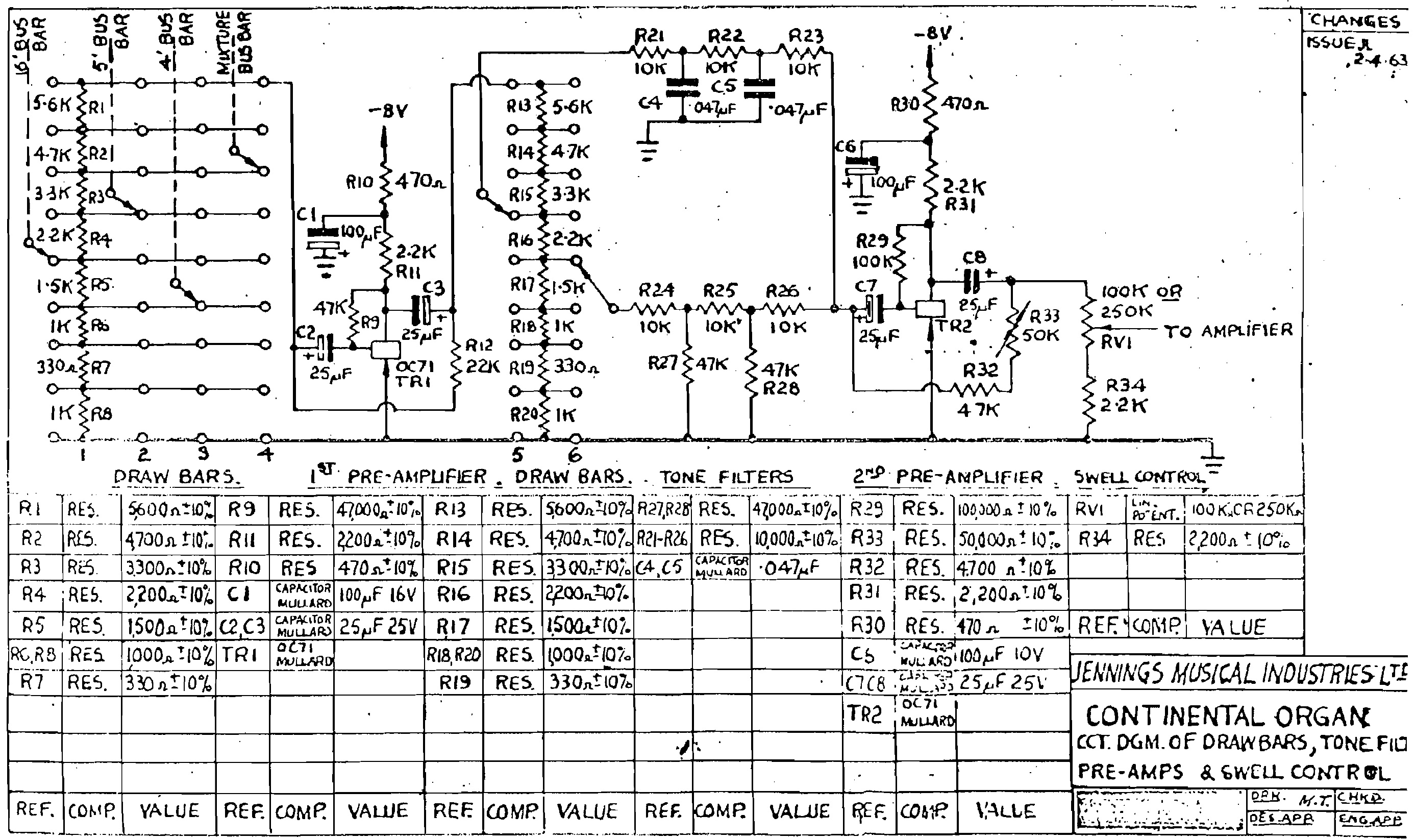
The third and final lesson was tuning. The Mostek MK50240 is driven by a crystal-controlled 2000.240 kHz master clock. The emulated “master clock” is determined by the speed of the non-terminating loop (cycling at the so-called “loop frequency”):
    for (;;) {
      if (--CnatCount == 0) {
        digitalWrite(CnatPin, (CnatState ^= 0x01)) ;
        CnatCount = CNAT ;
      }

      ...

      delaySum = delaySum + 1 ;
    }
My original plan was to tune all twelve pitches by changing the speed of the non-terminating loop. I discovered that such timing was too sensitive to code generation to be controllable and reliable. The biggest delay that I could add to the non-terminating loop was “delaySum = delaySum + 1 ;“. In the end, I manually tuned the individual note divisors.
A fine point: I chose the divisors to achieve a wide resolution in 8 bits. Eight bits is “close enough for rock and roll,” but not really enough for accurate tuning.
As usual, the path to the solution was zig-zaggy and not straight. Here is a ZIP file with all of the code and my working notes. I included source code for the intermediate experiments so you can re-trace my steps. Have fun!
Copyright © 2021 Paul J. Drongowski