If you read my posts about ARM Cortex-A72 micro-architecture:
you’re probably wondering, “How I do I reduce all of this to practice on Raspberry Pi 4?”
Program performance tuning is experimental and is measurement-based.
Our goal is to reduce program execution time by efficiently exploiting the underlying machine micro-architecture. Tuning follows a systematic, multi-step process:
- Initial design and code.
- Run and measure execution time and performance events.
- Analyze measurements.
- Make a hypothesis about performance bottlenecks.
- Change the code.
- Go to step 2 until you’re satisfied.
“Satisfied” is a bit subjective, but generally means “produces a result within a defined time constraint”, “achieves the desired frame rate,” or some other time-related design requirement.
You will need performance measurement tools and techniques. This is where hardware performance events come into play. Raspberry Pi OS is Linux, and fortunately, Linux has a mature performance measurement infrastructure. Performance Events for Linux, often called “PERF,” is the best way to get started. I’ve written extensively about PERF including my three part PERF tutorial:
- PERF tutorial: Finding execution hot spots
- PERF tutorial: Counting hardware performance events
- PERF tutorial: Profiling hardware events
The PERF tutorial illustrates performance measurement and tuning on Raspberry Pi models 1, 2 and 3. The mechanics of running PERF are the same on Raspberry Pi 4. Please see my other articles about Cortex-A72 performance tuning:
Lately, I have been experimenting with program performance self-monitoring using the Linux perf_event_open() system call. Stay tuned for more details and code. For the moment, I’m going to focus on ARM Cortex-A72 performance events — good enough to help you apply techniques and commands in the PERF tutorial.
Cortex-A72 performance events
A performance event is the occurrence of a micro-architectural condition. The simplest example events are retired instructions and processor (CPU) cycles. A retired instruction event occurs every time an instruction successfully completes (architectural) execution. A processor cycle event occurs every processor clock tick.
Each Cortex-A72 core has six performance counter registers. Using a tool like PERF, a performance event is assigned to each register. Yes, you can measure up to six performance events simultaneously, i.e., in a single experimental execution run. [More events can be measured via counter multiplexing, but I’m keeping things simple here.] The trick is to choose and configure the performance events that help you test your performance tuning hypothesis.
The ARM Cortex-A72 performance events are listed in the ARM Cortex-A72 Technical Reference Manual (TRM) available at the ARM corporate web site. The list is rather long and not all of the events are particularly relevant for application programmers. Thus, I won’t list them all here. There are several major event categories:
- Instructions and cycles
- Level 1 instruction (L1I) cache events
- Level 1 data (L1D) cache events
- Level 2 (L2) cache events
- Level 1 instruction TLB (L1 ITLB) events
- Level 1 data TLB (L1 DTLB) events
- Branches and mispredicted branches
- Bus and primary memory access
- Memory barriers (speculative)
- Instruction mix (speculative)
- Exceptions taken
- System register access
These are my own categories and should give you a rough impression about the kinds of micro-architectural events you can measure on Raspberry Pi 4. I listed the categories from highest to lowest priority placing the most relevant and generally useful event categories near the top of the list.
Each Coretex-A72 performance event type is assigned an event number. The event number identifies the event to measurement tools and to the event counting hardware.
Time and instruction events
Processor/CPU cycles and retired instructions are the true all-rounders.
Processor cycles are a good proxy for actual execution time. Sure, you can measure wall-clock or CPU execution time using the Linux time command or system calls like gettimeofday(), time(), clock() or clock_gettime(). The CPU cycle event lets us measure time using a performance counter register. The cycle count tells us approximately how much CPU time was consumed by the program under test.
As mentioned earlier, the retired instruction event counts the number of successfully (architecturally) completed instructions. Given a specific data set, every program has a specific amount of work to be accomplished. Particularly in the case of a single-threaded program, the program executes the same instructions for the same given data set, every time. Thus, the retired instruction count is a measure of work accomplished and should be (roughly) the same every experimental run, assuming the same data set and no outside interference. (You shouldn’t run other applications while testing. Control the test environment!)
    Number  Mnemonic      Name
    ------  ------------  ------------------------------------
    0x08    INST_RETIRED  Instruction architecturally executed
    0x11    CPU_CYCLES    Cycle
    0x1B    INST_SPEC     Operation speculatively executed
Instructions per cycle (IPC)
Two basic performance tuning goals are:
- Reduce the number of processor cycles, and
- Reduce the number of retired instructions.
Reducing the number of processor cycles should reduce the overall execution time. That assumes, of course, that overall execution time is not dominated by input/output, page faults, human wait (interaction) time, or some other major factor!
Reducing the number of retired instructions should reduce the amount of work performed by the program. Optimizing compilers work hard to reduce the number of instructions in tight inner loops. In terms of conventional wisdom, the fastest instruction is an instruction which is never executed in the first place.
Practically, however, one program can execute more instructions and achieve a shorter execution time than another program (assuming the same data set and functionality, of course). How can this be? It comes down to a few fundamental factors:
- Read and use data from fast cache memory.
- Reducing reads (writes) from (to) slow primary memory.
- Execute computations concurrently.
- Overlap execution with read and write operations.
Short answer, it comes down to exploiting instruction-level parallelism (ILP), temporal data locality and spatial data locality.
Instructions per cycle (IPC) is one simple measure that tells us how we are doing overall. IPC is easy to measure and compute: Count the number of retired instructions, count the number of processor cycles, and divide:
INST_RETIRED / CPU_CYCLES
The IPC ratio indicates the amount of useful work done during each processor cycle and we want to maximize it.
Goal IPC is very much application dependent. For a given critical inner loop, one might ask, “How many concurrent operations (computations, reads, writes) can Cortex-A72 perform assuming the data are cache-resident?” If IPC is significantly less than one, it’s probably time to tune. In scientific code with a mix of integer and floating point operations, an IPC of 2 is a good starting goal.
Speculative execution
ARM Cortex-A72 is a superscalar processor which predicts branch direction and executes instructions speculatively along predicted program paths. The A72 is capable of counting many speculative event types. Speculative event types are explicitly identified in the ARM Cortex-A72 Technical Reference Manual; Look for “_SPEC” in the event mnemonic.
The speculated instruction event count is the number of ARMv8-A issued
speculatively during program execution. Ideally, branch predictions are always correct and every speculatively issued instruction eventually retires. Speculatively issued instructions on a wrong path consume execution resources just like correct path instructions that retire. Unfortunately, wrong path results are discarded, thereby wasting any resources which they consumed. Fewer wrong-path instructions produces less waste, that is, fewer wrong-path instructions start execution, consume resources, and are discarded.
The ratio of speculated instructions to retired instructions:
INST_RETIRED / INST_SPEC
indicates how often speculated instructions resolved into retirement. Best case, this ratio is one — all speculated instructions eventually retired (i.e., few execution resources are wasted).
Example: Matrix multiplication
Matrix multiplication is the classic example of performance tuning for micro-architecture. Mathematics specifies the end result — the matrix product. Algorithmically, however, there are two ways to compute the matrix product:
- Textbook algorithm and code: Straightforward implementation of the mathematics.
- Loop nest interchange algorithm and code: Cache-friendly implementation which exploits temporal and spatial locality.
For more detail about the algorithms and code, please see Textbook matrix multiplication (part 1) and Faster matrix multiplication (part 2).
I ran both the textbook and loop nest interchange programs on Raspberry Pi 4. The textbook code took 28.6 seconds and, as expected, the interchange code took more time, 19.6 seconds. Here are the raw event counts:
    Event                    Textbook        Interchange
    -----------------------  --------------  --------------
    Retired instructions     38,227,831,497  60,210,830,503
    CPU cycles               42,041,568,760  29,332,934,027
    Instructions per cycle   0.909           2.053
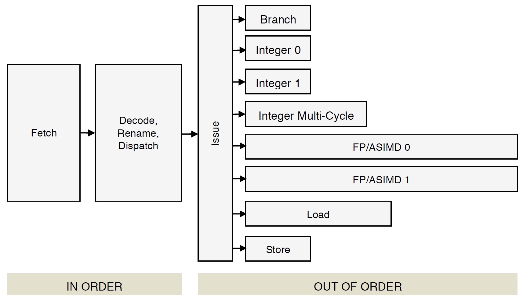
The textbook program executed less than one instruction per processor cycle, 0.909 IPC. The textbook code underperforms with respect to the availability of Cortex-A72 execution units (two integer, two FP units) and the opportunity to overlap computation with memory access. The interchange program achieves a respectable 2.053 instructions per cycle. The interchange version consumes far fewer processor cycles than the textbook version.
Just for grins, multiply the CPU cycle counts by the Raspberry Pi 4 clock period (the inverse of the 1.5GHz clock frequency). You get approximately the measured
clock()CPU times: 28.028 seconds versus 28.6 actual and 19.555 seconds vs. 19.6 seconds actual.
Here are the raw event counts for retired and speculated instructions:
    Event                    Textbook        Interchange
    -----------------------  --------------  --------------
    Retired instructions     38,227,831,497  60,210,830,503
    Speculated instructions  46,576,925,991  60,254,256,720
    Retired / speculated     0.821           0.999
The interchange version has a near ideal retired to speculated instruction ratio (0.999). The textbook slightly underperforms with nearly 8 million speculated instructions started and abandoned.
The programs are written in C and compiled with the -O0 optimization level. Try -O3. The results may further surprise you. 🙂
Copyright © 2021 Paul J. Drongowski