I’m in the midst of investigating a performance anomaly which seemingly pops up at random. I wrote a pointer chasing program to exercise and measure cache miss performance events. As part of the testing regimen, I run the program several times in a row and compare run time, event counts, etc. and look for inconsistencies.
The program is usually well-behaved/consistent and produces the expected result. For example, when the program is configured to always hit in the level 1 data (L1D) cache, the program measures just a few L1D misses and the run time is short. However, occasionally a run is slow and has a slew of L1D misses. What’s up?
My first thought was re-scheduling, that is, the pointer chasing program starts on one core and is moved by the OS to another core. The cache on the new core is cold and more misses occur. The Linux taskset command launches and pins a program to a core. In fancier language, it sets the CPU affinity for a (running) process. If we pin the program to a particular core, the cache should stay warm.
If you’re an old-timer and haven’t used taskset in a while, please be aware that a user must have CAP_SYS_NICE capability to change the affinity of a process. You can also set CAP_SYS_NICE capability for an application binary using the setcap utility:
sudo setcap 'cap_sys_nice=eip' <application>
You can check capabilities with getcap:
getcap <application>
The form of the capabilities string is in accordance with the cap_from_text call, so I recommend viewing its man page. The eip flags are case sensitive and specify the effective, inheritabe and permitted sets, respectively.
As to the performance anomoly, setting the CPU (core) affinity did not resolve the issue. Long runs and misses kept popping up. My next thought was “maybe CPU clock throttling?”
There’s quite a bit of on-line material about Raspberry Pi clock throttling and I won’t repeat all of it here. Suffice it to say, the RPi 4 firmware has a so-called CPU scaling governor that kicks in at high temperatures. The governor tries to keep the CPU temperature below 80℃ . Over-temperature occurs when the temperature rises above 85℃ . The governor adjusts (throttles) the CPU clock to achieve the configured operating temperature goals.
We do know that Raspberry Pi 4 can run hot. My RPi4 has heat sinks installed, but no case fan. Heat vents out the top of the Canakit plastic enclosure. The heat sinks are warm to the touch, not super hot, really. However, it’s not a bad idea to take the Pi’s temperature.
The following command displays the RPi’s temperature:
cat /sys/class/thermal/thermal_zone0/temp
Divide the result by 1000 to obtain the temperature in degrees Celsius. The next command displays the current frequency (kHz):
Divide the result by 1000 to obtain the frequency in MHz. This frequency is the Linux kernel’s requested frequency. The actual, possibly throttled frequency may be different.
The Pi’s vcgencmd command is even better! vcgencmd is the Swiss Army knife of system info utilities. The following command displays a list of vcgencmd subcommands:
vcgencmd commands
Here’s a few commands to get you started:
    vcgencmd measure_temp
    vcgencmd measure_clock arm
    vcgencmd measure_volts core
    vcgencmd get_throttled
You may run into permission issues with vcgencmd. I couldn’t tame the permissions and simply ran vcgencmd via sudo.
The get_throttled subcommand returns a bit mask. Here’s the magic decoder ring:
    Bit   Hex value  Meaning
    ----  ---------  -----------------------------------
    0     1          Under-voltage detected (< 4.64V)
    1     2          Arm frequency capped (temp > 80'C)
    2     4          Currently throttled
    3     8          Soft temperature limit active
    16    10000      Under-voltage has occurred
    17    20000      Arm frequency capping has occurred
    18    40000      Throttling has occurred
    19    80000      Soft temperature limit has occurred
If all of that isn’t enough, you can install and run cpufrequtils:
    sudo apt install cpufrequtils
    cpufreq-info
After running the workload and measuring both CPU clock and temperature, throttling did not appear to be a problem. My current conjecture has to do with Linux fixes for the Spectre security vulnerability. In short, Spectre is a class of vulnerabilities exploiting observable side-effects of the machine micro-architecture in order to set up clandestine information channels that leak confidential data. One way to supress data cache observables is to flush (clean) and invalidate the data caches during a context switch. If the data cache is invalidated, cache misses and program run time will go up. Stay tuned.
Even though I haven’t found the source of the performance anomoly, I welcomed the chance to learn about vcgencmd, etc. Off to investigate Linux hardware cache flushing…
Back on the old day job, I developed and tested software and hardware for program profiling. Testing may sound like drudge-work, but there are ways to make things fun!
Two questions arise while testing a profiling infrastructure — software plus hardware:
Does the hardware accurately count (or sample) performance events for a given specific workload?
Does the software accurately display the counts or samples?
Clearly, ya need working hardware before you can build working software.
Testing requires a solid, known-good (KG) baseline in order to decide if new test results are correct. Here’s one way to get a KG baseline — a combination of static analysis and measurement:
Static analysis: Analyze the post-compilation machine code and predict the expected number of instruction retires, cache reads, misses, etc.
Measurement: Run the code and count performance events.
Validation: Compare the measured results against the predicted results.
Thereafter, one can compare new measurements taken from the system under test (SUT) and compare against both predicted results and baseline measured results.
Applying this method to performance counter counting mode is straightforward. You might get a little “hair” in the counts due to run-to-run variability, however, the results should be well-within a small measurement error. Performance counter sampling mode is more difficult to assess and one must be sure to collect a statistically significant number of samples within critical workload code in order to have confidence in a result.
One way to make testing fun is to make it a game. I wrotekernel programs that exercised specific hardware events and analyzed the inner test loops. You could call these programs “test kernels.” The kernels are pathologically bad (or good!) code which triggers a large number of specific performance events. It’s kind of a game to write such bad code…
The expected number of performance events is predicted through machine code level complexity analysis known as program “microanalysis.” For example, the inner loops of matrix multiplication are examined and, knowing the matrix sizes, the number of retired instructions, cache reads, branches, etc. are computed in closed form, e.g.,
This formula is the closed form expression for the retired instruction count within the textbook matrix multiplication kernel. The microanalysis approach worked successfully on Alpha, Itanium, x86, x64 and (now) ARM. [That’s a short list of machines that I’ve worked on. 🙂 ]
With that background in mind, let’s write a program kernel to deliberately cause branch mispredictions and measure branch mispredict events.
The ARM Cortex-A72 core predicts conditional branch direction in order to aggressively prefetch and dispatch instructions along an anticipated program path before the actual branch direction is known. A branch mispredict event occurs when the core detects a mistaken prediction. Micro-ops on the wrong path must be discarded and the front-end must be steered down the correct program path. The Cortex-A72 mispredict penalty is 15 cycles.
What we need is a program condition that consistently fools the Cortex-A72 branch prediction hardware. Branch predictors try to remember a program’s tendency to take or not take a branch and the predictors are fairly sensitive; even a 49%/51% split between taken and not taken has a beneficial effect on performance. So, we need a program condition which has 50%/50% split with a random pattern of taken and not taken direction.
Here’s the overall approach. We fill a large array with a random pattern of ‘0’ and ‘1’ characters. Then, we walk through the array and count the number of ‘1’ characters. The function initialize_test_array() fills the array with a (pseudo-)random pattern of ones and zeroes:
void initialize_test_array(int size, char* array,
               int always_one, int always_zero)
{
    register char* r = array ;
    int s ;
    for (s = size ; s > 0 ; s--) {
        if (always_one) {
            *r++ = '1' ;
        } else if (always_zero) {
            *r++ = '0' ;
        } else {
            *r++ = ((rand() & 0x1) ? '1' : '0') ;
        }
    }
}
The function has options to fill the array with all ones or all zeroes in case you want to see what happens when the inner conditional branch is well-predicted. BTW, I made the array 20,000,000 characters long. The size is not especially important other than the desire to have a modestly long run time.
The function below, test_loop(), contains the inner condition itself:
int test_loop(int size, char* array)
{
    register int count = 0 ;
    register char* r = array ;
    int s ;
    for (s = size ; s > 0 ; s--) {
        if (*r++ == '1') count++ ;    // Should mispredict!
    }     return( count ) ;
}
The C compiler translates the test for ‘1’ to a conditional branch instruction. Given an array with random ‘0’ and ‘1’ characters, we should be able to fool the hardware branch predictor. Please note that the compiler generates a conditional branch for the array/loop termination condition, s > 0. This conditional branch should be almost always predicted correctly.
The function run_the_test() runs the test loop:
void run_the_test(int iteration_count, int array_size, char* array)
{
  register int rarray_size = array_size ;
  register char* rarray = array ;
  int i ;
  for (i = iteration_count ; i-- ; ) {
      test_loop(array_size, array) ;
  }
}
It calls test_loop() many times as determined by iteration_count. Redundant iterations aren’t strictly necessary when taking measurements in counting mode. They are needed, however, in sampling mode in order to collect a statistically significant number of performance event samples. I set the iteration count to 200 — enough to get a reasonable run time when sampling.
The test driver code initializes the branch condition array, configures the ARM Cortex-A72 performance counters, starts the counters, runs the test loop, stops the counters and prints the performance event counts:
The four counter configuration, control and display functions are part of a small utility module that I wrote. I will explain the utility module in a future post and will publish the code, too.
Finally, here are the measurements when scanning an array holding a random pattern of ‘0’ and ‘1’ characters:
Please recall that there are two conditional branches in the inner test loop: a conditional branch to detect ‘1’ characters and a conditional branch to check the array/loop termination condition. The loop check should be predicted correctly almost all the time, accounting for 50% of the total number of correctly predicted branches. The character test, however, should be incorrectly predicted 50% of the time. It’s like guessing coin flips — you’ll be right half the time on average. Overall, 25% of branch predictions should be incorrect, and yes, the measured branch mispredict ratio is 0.250 or 25%.
The number of speculated instructions is also very interesting. Cortex-A72 speculated twice as many ARMv8 instructions as it retired. Over half of the speculated instructions did not complete architecturally and were discarded. That’s what happens when a conditional branch is grossly mispredicted!
In my discussion about instructions per cycle as a performance metric, I compared the textbook implementation of matrix multiplication against the loop next interchange version. The textbook program ran slower (28.6 seconds) than the interchange version (19.6 seconds). The interchange program executes 2.053 instructions per cycle (IPC) while the textbook version has a less than stunning 0.909 IPC.
Let’s see why this is the case.
Like many other array-oriented scientific computations, matrix multiplication is memory bandwidth limited. Matrix multiplication has two incoming data streams — one stream from each of the two operand matrices. There is one outgoing data stream for the matrix product. Thanks to data dependency, the incoming streams are more important than the outgoing matrix product stream. Thus, anything that we can do to speed up the flow of the incoming data streams will improve program performance.
Matrix multiplication is one of the most studied examples due to its simplicity, wide-applicability and familiar mathematics. So, nothing in this note should be much of a surprise! Let’s pretend, for a moment, that we don’t know the final outcome to our analysis.
I measured retired instructions, CPU cycles and level 1 data (L1D) cache and level 2 (L2) cache read events:
There is one big take-away here. The textbook program misses in the data cache far more often than interchange. The textbook L1D cache miss ratio is 0.073 (7.3%) while the interchange cache miss ratio is 0.001 (0.1%). As a consequence, the textbook program reads the slower level 2 (L2) cache more often to find necessary data.
If you noticed slightly different counts for the same event, good eye! The counts are from different runs. It’s normal to have small variations from run to run due to measurement error, unintended interference from system interrupts, etc. Results are largely consistent across runs.
The behavioral differences come down to the memory access pattern in each program. In C language, two dimensional arrays are arranged in row-major order. The textbook program touches one operand matrix in row-major order and touches the other operand matrix in column-major order. The interchange program touches both operand arrays in row-major order. Thanks to row-major order’s sequential memory access, the interchange program finds its data in level 1 data (L1D) cache more often than the textbook implementation.
There is another micro-architecture aspect to this situation, too. Here are the performance event counts for translation look-aside buffer (TLB) behavior:
    Event                          Textbook     Interchange
    -----------------------  --------------  --------------
    Retired instructions     38,227,830,517  60,210,830,503
    L1 D-cache reads         15,070,845,178  19,094,937,273
    L1 DTLB miss              1,001,149,440          17,556
    L1 DTLB miss LD           1,000,143,621          10,854
    L1 DTLB miss ST               1,005,819           6,702
Due to the chosen matrix dimensions, the textbook program makes long strides through one of the operand matrices, again, due to the column-major order data access pattern. The stride is big enough to touch different memory pages, thereby causing level 1 data TLB (DTLB) misses. The textbook program has a 0.066 (6.6%) DTLB miss ratio. The miss ratio is near zero for the interchange version.
I hope this discussion motivates the importance of cache- and TLB-friendly algorithms and code. Please see the following articles if you need to brush up on ARM Cortex-A72 micro-architecture and performance events:
Here is a list of the ARM Cortex-A72 performance events that are most useful for measuring memory access (load, store and fetch) behavior. Please see the ARM Cortex-A72 MPCore Processor Technical Reference Manual (TRM) for the complete list of performance events.
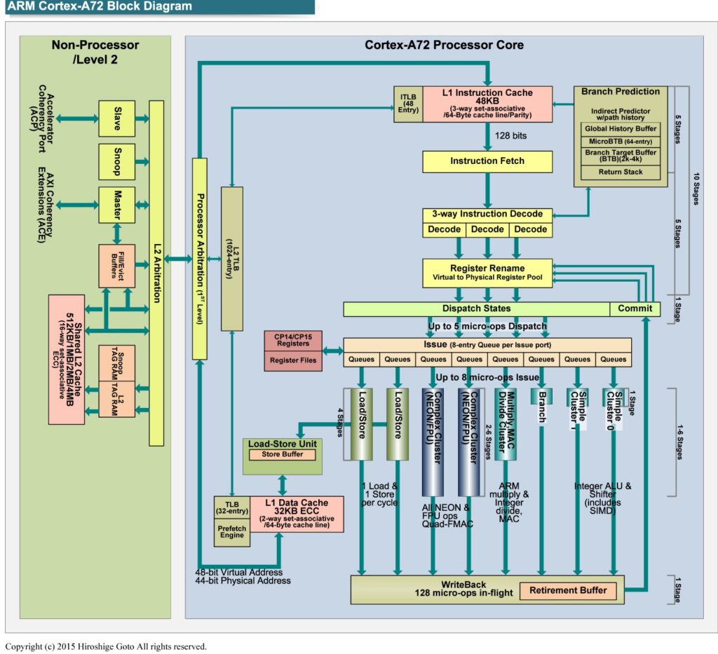
The Cortex-A72 front-end puts micro-ops into per-pipe issue queues which, in turn, feed the execution units. There are eight issue queues. The queues have eight entries each except the branch queue, which has ten entries (66 queue entries total like the old Cortex-A57). The queues provide rate-balancing between the core front-end (i.e., the instruction/micro-op stream) and the execution units. The queues allow greater parallelism between units, too, letting each pipeline run at its own independent single- or multi-cycle speed.
ARM Cortex-A72 micro-architecture (Source: Hiroshige Goto)
The branch and integer pipes are very fast, each pipe executing a micro-op in a single processor cycle. The integer pipelines have multiple, zero-cycle forwarding datapaths. These paths, sometimes called “by-passes,” send intermediate results directly to stages (computations) needing the result right darned now without writing the result into the rename register file first.
The integer multi-cycle pipe handles integer micro-ops which require 2 or more processor cycles for execution. Shift operations are relatively fast: 2+ cycles. Integer multiplication has a 3 to 5 cycle latency. Integer divide is relatively slow taking anywhere from 4 to 20 cycles. Multiplication can be accelerated through dedicated combinational logic; division is sequential by nature and requires many steps.
The FP (floating point) and ASIMD (Advanced Single Instruction Multiple Data) units perform floating point and SIMD computations. Both units are generalist and perform commonly occurring FP operations: FP ADD, SUB, MUL, NEG, ABS, MAX, MIN, etc. Execution latency varies from 3 to 4 cycles for these basic operations. The FP pipes support late forwarding of FP MUL products to FP multiply-accumulate micro-ops, letting FP multiply-accumulate complete in 6 cycles.
Each FP unit is a specialist, too:
FP/ASIMD 0: FP CONVERT, ROUND, DIV, CRYPTO
FP/ASIMD 1: FP COMPARE, SQRT
FP divide and square root operations are performed using iterative algorithms. Only one FP DIV or SQRT operation at a time may execute in a pipe. Latencies are long: 6 to 18 cycles for DIV and 6 to 32 cycles for SQRT, depending upon FP datatype.
Please see the ARM Cortex-A72 Software Optimization Guide for detailed instruction timing, pipe assignment and ASIMD operation.
Load and store micro-ops are executed by the load and store units. The load and store units are mutually independent. One load and one store micro-op can execute each processor cycle. (Load and store are discussed below.) Load and store micro-ops issue speculatively. Under speculative execution, a load or store may reside on a correctly predicted branch path (the correct path) or an incorrectly predicted branch path (the wrong path). Loads, stores and associated data on a wrong path must be discarded. Store operations are buffered (wait) until they are determined to be on the correct path and are committed architecturally to primary memory.
Memory hierarchy
As I mentioned in my Cortex-A72 overview, the Raspberry Pi 4 (Broadcom BCM2711) has a four level memory hierarchy:
          Register          Fast, but small
              |
        Level 1 caches
              |
        Level 2 cache
              |
             RAM             Big, but slow
The RPi4 has four A72 cores. Each core has a register file and level 1 instruction and data caches. The four cores share a single unified level 2 cache and primary memory (RAM).
The register file is the fastest, but has the smallest capacity. Registers are read or written in a single processor cycle. RAM has the most capacity, but is relatively slow. RPi4 primary memory is LPDDR4-3200 SDRAM:
The following table summarizes Cortex-A72 cache characteristics:
L1I cache capacity
48KB
L1I cache organization
Per-core, 3-way set associative, 64B line
L1D cache capacity
32KB
L1D cache organization
Per-core, 2-way set associative, 64B line
L2 cache capacity
1MB
L2 cache organization
Shared, 16-way set associative, 64B line
Data accesses are handled by the Level 1 Data (L1D) cache. Instruction fetches are handled by the Level 1 Instruction (L1I) cache. The Level 2 (L2) cache is unified, handling both data and instructions. The Raspberry Pi BCM2711 ARM Peripherals manual states the following caveat with respect to the L2 cache:
BCM2711 provides a 1MB system L2 cache, which is used primarily by the GPU. Accesses to memory are routed either via or around the L2 cache depending on the address range being used.
Thus, application programs should not expect to receive a performance assist from the L2 cache! The VideoCode GPU accesses L2 cache through the Cortex-A72 ACP/AXI interface.
The L1D cache load-to-use latency is 4 cycles when the load hits in the L1D cache. The Level 2 (L2) cache load-to-use latency is 9 cycles when the load hits in the L2 cache.
A read access (e.g., a data load or instruction fetch) first tries the appropriate level 1 cache (Load: L1D cache, Fetch: L1I cache). If it finds the requested item in the level 1 cache — a hit — the item is sent to either the rename registers (for loads) or the instruction decoder (for fetches). Load data may also be sent through a bypass to an execution stage (micro-op) awaiting the incoming data.
If the read access misses the level 1 cache, the request is sent (optionally) to the unified L2 cache. If the requested item is found in L2 cache, the cache line containing the item is written into the level 1 cache, thereby replacing one of the existing lines. This operation is called a “refill.” If the line to be replaced is dirty (modified), then the old value is evicted and is written to primary memory. The requested item is selected from the incoming cache line and is routed to the appropriate destination (i.e., functional unit or instruction decoder).
If the read access misses (or optionally, bypasses) the L2 cache, the 64 byte line containing the item is read from primary memory. The incoming line is written to the level 1 cache (a refill) and (optionally) the L2 cache. Again, dirty lines are evicted.
Instruction and data bytes are read, written and transferred in 64-byte chunks (lines). This is true even if a load instruction requests a single byte from memory. Application programs should strive to use each entire cache line completely before moving on to the next line. Programs that exploit spatial and temporal locality perform better. Programmers need to pay careful attention to algorithm selection, data structure/layout and memory access patterns in order to make good, efficient use of data caching.
The description of Cortex-A72 cache operation above is simplified. Consider, for example, memory transaction types. Memory attributes within the Memory Management Unit (MMU) and page tables determine memory transaction types for each memory region:
Write-Back Read-Write-Allocate
Write-Back No-Allocate
Write-Through
Non-cacheable
Device
Memory transaction type affects cache behavior.
Write-Back Read-Write-Allocate is the most common and highest performing memory type. Incoming lines are written to the L1D cache and the read (or write) completes from the L1D cache. A store that hits a Write-Back cache line does not update main memory.
Write-Back No-Allocate does not write an incoming line to L1D cache. This prevents cache pollution when accessing large, one-time use data structures.
Non-cacheable memory bypasses both the level 1 caches and L2 cache. Requests go directly to primary memory. The Cortex-A72 treats Write-Through memory as Non-cacheable.
Instruction fetch (more details)
Instruction fetches are speculative and there is no guarantee that fetched instructions are executed. Instructions are aggressively prefetched pursuing either sequential execution flow or branch targets based on path prediction.
The L1I cache is fed by three fill buffers that hold instructions from either the unified L2 cache or primary memory. The fill buffers are non-blocking. A line may remain in a fill buffer until it is transferred to the L1I cache or discarded. Primary memory regions may be marked as non-cacheable regions or the L1I cache may be disabled, and incoming lines are not written to the L1I cache. A line is not committed to the L1I cache unless it is demanded by a fetch. The hardware also has an L2 instruction prefetcher.
Cortex-A72 treats the preload instruction cache instruction (PLDI) as a NOP.
Memory Management Unit
The Memory Management Unit (MMU) performs virtual to physical address translation and enforces secure, restricted access to memory regions. As to security, suffice it to say that the MMU restricts access by Address Space Identifier (ASID) and Virtual Machine Identifier (VMID). These concerns are addressed by the operating system and are generally transparent to application programmers. [And I won’t be dealing with access control here.]
Address type
AArch64
AArch32
Virtual address (VA)
48 bits
32 bits
Physical address (PA)
44 bits
40 bits
The Cortex-A72 hardware supports 4KB, 64KB and 1MB page sizes. The Raspberry Pi Operating System (formerly known as “Raspbian”) organizes primary memory into 4KByte pages. [Huge pages must be enabled in the kernel and I will assume that it’s 4KB all the way on RPi4.] The operating system maintains page tables that specify the physical location of application program pages (both instructions and data).
Application programs use virtual addresses to identify instructions and data items. Conceivably, hardware could use memory-resident page tables to map a virtual address to its corresponding physical address. This approach is way too slow to be practical. Better, the Cortex-A72 maintains page (address) mapping information in a multi-level, hierarchical memory system:
       Level 1 TLB          Fast, but small
            |
       Level 2 TLB
            |
           RAM              Big page tables, but slow
The TLB structure is separate from the register/cache/memory hierarchy and it operates independently. The organizing principle is the same — most recent and frequently used mappings reside in fast memory and big page tables reside in slow primary memory.
“TLB” is the acronym for “translation lookaside buffer.” A TLB is an array where each entry describes the mapping from a virtual page to a physical page. Internal operation of a TLB is similar to a data cache. The following table summarizes Cortex-A72 TLB characteristics:
L1I TLB capacity
48 entries
L1I TLB organization
Fully associative
L1D TLB capacity
32 entries
L1D TLB organization
Fully associative
L2 TLB capacity
1024 entries
L2 TLB organization
4-way set associative
The L1I and L2D TLBs support 4KB, 64KB, and 1MB page sizes. The L2 TLB supports 4KB, 64KB, 1MB and 16MB page sizes. (Also, 2MB and 1GB using AArch32 long descriptor format translation.) Alas, Raspberry Pi OS uses 4KB pages.
TLB operation is similar to caching. Address translation is first tried in the L1I TLB (fetches) or L1D TLB (loads and stores). If the translation information is found (a hit), the physical address is returned in one cycle. Access permission is checked at the same time.
If translation misses in a level 1 TLB, address translation is attempted in the main L2 TLB. If the translation information is found, the physical address is returned (after one or more cycles).
If translation misses in the L2 TLB, the MMU performs a hardware translation table walk. (Page tables have a fairly complicated structure which is beyond the scope of this discussion.) Because page tables reside in slow primary memory, a hardware translation table walk takes a relatively long time to complete with respect to an L2 TLB look-up.
If the required page is not in memory and is on the RPi OS swap device, the operating system reads the page into primary memory before attempting re-translation. These exceptions, page faults, are the slowest of all and they should be avoided like the plague.
Once again, program performance depends up good temporal and spatial locality, albeit locality at the page level. An application program can touch as many as 32 different data pages without triggering an L1D TLB refill:
32 L1D TLB entries * 4 KBytes/page = 128 KByte data working set
This is a modest-sized working set of pages, and like cache line strategy, a program should make maximal, efficient use of a page working set before demanding new page translation information from the L2 TLB. The L2 TLB supports a larger combined data/instruction working set:
1024 L2 TLB entries * 4 KBytes/page = 4 MByte total working set
The L2 TLB footprint (working set size) is larger. However, the L1D TLB and the L1I TLB compete for page translation entries in the unified L2 TLB.
As to data-page utilization, data structure layout and access pattern come into play once again. A program should work as much as possible within the current working set before moving to pages outside the current set. Random access within a big heap pays a penalty when heap items are distributed across many pages (i.e., when the working set exceeds 32 pages).
With respect to L1I TLB utilization strategy, frequently executed, related code should reside within the same page or just a few pages. Related code which is spread across many pages (i.e., a large instruction working set) will jump between pages and possibly cause L1I TLB or L2 TLB refills.
The above description of the translation process is simplified. For example, access is checked against page permissions, etc. and violations are reported after aborting offending translation and instruction. I tried to focus mainly on performance-related concerns of interest to application programmers.
Load and store operations
After absorbing all of that, let’s pick up a few additional odds and ends about load and store operations.
Cortex-A72 memory operations are weakly ordered. They may be performed out-of-order as long as data dependencies are honored. Due to the weak ordering, explicit synchronization barriers are needed in circumstance where strong ordering is required. There are four kinds of barriers:
Instruction Synchronization Barrier (ISB)
Data Synchronization Barrier (DSB)
Data Memory Barrier (DMB)
Load-Acquire (LDAR) and Store-Release (STLR)
Please see the Programmer’s Guide for ARMv8-A for further details.
More generally important to application programmers is data alignment. Naturally aligned data is accessed faster than unaligned data, especially unaligned data items that cross cache line boundaries. The following table summarizes alignment requirements:
Source: Programmer’s Guide for ARMv8-A
Load operations should not cross 64-byte, cache line boundaries. Store operations should not cross 16-byte boundaries.
As a general program design principle, computations proceed as fast as data items can stream from primary memory, and secondarily, as fast as results can stream back to primary memory. Data prefetching increases the speed of incoming data stream(s). The programmer or compiler should schedule load operations further ahead of instructions which consume the incoming data item. Ideally, other independent instructions are scheduled and executed ahead of the consuming load thereby overlapping useful computation with load latency (4 cycles from the L1D cache at a minimum).
A program may signal the need for a data item through an explicit prefetch instruction. The A72 supports three instruction prefetch hint instructions: PLD, PLDW, and PRFM. These are only hints and may be ignored. The PLD and PLDW instructions allocate a line in the Level 1 Data cache. Prefetch from Memory (PRFM) hints that data from a specific address will soon be needed. If accepted, these hints can bring in a data item (cache line) before it is required.
Programmers may further manage data cache contents via non-temporal load and store instructions (LDNP and STNP). These instructions hint that caching is not useful for data at an address, thereby preventing unnecessary cache pollution. Non-temporal load and store instructions may require explicit load barriers. (See the Programmer’s Guide for ARMv8-A for more details.)
The Cortex-A72 hardware has a load-side prefetcher which dynamically analyzes memory access patterns. Based on its analysis, the load-side prefetcher brings data into either the L1D cache, the L2 cache, or both. The hardware also has a store-side prefetcher which brings data into the L2 cache.
Outgoing data streams benefit from write combining which merges data from multiple store operations into a single memory write access.
Outstanding read and write requests (i.e., pending requests to primary memory) wait in the Fill/Eviction Queue (FEQ). The Cortex-A72 has a configurable FEQ: 20, 24, or 28 entries. The A72 write issuing capability is 16, that is, up to 16 writes may be outstanding at any time. The read issuing capability is 19, 23, or 27 depending upon FEQ configuration (capacity). L2 prefetch is throttled based on the FEQ occupancy count. [Extra credit: What is the specific Raspberry Pi 4 FEQ configuration and occupancy threshold?]
One important simplification in the cache discussion is cache coherency. Most application programmers needn’t worry about cache coherency. However, if you are writing a program with multiple, co-operating threads that actively share memory locations or regions, you should MOESI over to the ARM Cortex-A72 Technical Reference Manual (TRM) and read up on the details. The A72 Snoop Control Unit (SCU) uses a hybrid protocol (MESI+MOESI) to maintain coherency between the per-core L1 data caches (MESI) and the common L2 cache (MOESI). “MESI” and “MOESI” refer to the coherency status of each cache line:
Modified (M)
Owned (O)
Exclusive (E)
Shared (S)
Invalid (I)
The BCM2711 employs an Advanced Microcontroller Bus Architecture (AMBA) Advanced xExtensible Interface (AXI) bus interface. Broadcom does not specify if either AXI Coherency Extensions (ACE) or the Coherency Hub Interface (CHI) are supported. (Man, these acronyms stack up!) Since ACE and CHI are intended for SMP processor clusters (e.g., big.LITTLE) these features may have been left out or disabled.
If you do care about cache coherency, please be aware that load data may be sourced from a remote L1D cache as well as the shared L2 cache or primary memory.
Sources
Before closing, I want to offer a few words about my sources. My primary resources are:
ARM Cortex-A72 Technical Reference Manual (TRM)
ARM Cortex-A72 Software Optimization Guide
ARM Programmer’s Guide for ARMv8-A
BCM2711 ARM Peripherals
These resources are authoritative. I also relied upon ARM’s own briefings and presentations about Cortex-A72 as found on the Web. I tried to verify Web sources and briefings against the written TRM and programmer guides.
In closing
Hopefully, my write-ups will help developers tune their programs for ARM Cortex-A72. If you’re just getting started with performance tuning, I would first concentrate on cache- and page-friendly algorithms, data structures and access patterns. Fill buffers, FEQ, memory ordering, and memory transaction types are esoteric subjects for most application programmers.
Want to learn more about Raspberry Pi 4 (Cortex-A72 / Broadcom BCM2711) performance tuning? Please read:
[Be sure to visit Living Computers in Seattle. SIGCSE 2017 attendees are admitted free during the conference. I visited the museum today and it was a lot of fun! K-12 teachers will enjoy the hands on exhibits.]
The annual ACM Special Interest Group on Computer Science Education (SIGCSE 2017) Technical Symposium is next week (March 8 – 11) in Seattle, Washington. The symposium brings together educators at all levels (K-12 and higher ed) to exchange and discuss the latest methods, practices and results in computer science education.
I don’t often advertise it, but the Sand, Software, Sound site has many resources for educators and students alike. You can browse these resources by clicking on one of the WordPress topic buttons (Raspberry Pi, PERF, Courseware, etc.) above. You can also search for a topic or choose from one of the categories listed in the right sidebar.
Here are a few highlights.
I taught many computer-related subjects during my career and have posted course notes, slides and old projects. The four main sections are:
CS2 data structures: Undergraduate data structures course suitable for advanced placement students.
Computer design: Undergraduate computer architecture and design which uses a multi-level modeling approach.
VLSI systems: Graduate course on VLSI architecture, design and circuits which is suitable for undergraduate seniors.
Please feel free to dig through these materials and make use of them.
Software and hardware performance analysis formed a major thread throughout my professional life. I recommend reading my series of tutorials on the Linux PERF tool set for software performance analysis:
The ARM11 microarchitecture summary is background material for the PERF tutorial. Program profiling is a good way to bring computer architecture to life and to teach students how to analyze and assess the execution speed of their programs.
There are two additional tutorials and getting started guides for teachers and students working on Raspberry Pi:
Music technology and computer-based music-making have been two of my chief interests over the years. The Arduino section of the site has several of my past projects using the Arduino for music-making. You should also check out my recent blog posts about the littleBits synth modules and littleBits Arduino. Please click on the tags and links at the bottom of each post in order to chase down material.
A new article on the Raspberry Pi (Broadcom BCM2835) memory hierarchy is almost ready. The first code has already been posted.
I’ve been working on multi-core processors for so long that I forgot what it’s like to take measurements on a single core machine like the Raspberry Pi.
In the ideal world, a benchmark or performance test program has the machine to itself and no other program or system activity perturbs it. Measurements on the ideal machine accurately and exactly reflect the dynamic behavior and performance of the program. On multi-core, you can usually assign the test program to an idle core (or two), preferably a core that is free of operating system activity. With careful process or thread placement, results on multi-core approach the ideal.
On single core, we don’t have any luxury. The test program has to share the one core with other programs and the operating system. On Raspberry Pi, Linux fires up services that run periodically. Even if we shut the services off, the system clock continues to run and it generates interrupts. At the very least, extraneous activity affects elapsed, user and system time measurements.
When we measure performance events, however, there is a deeper level of interference. The core has one physical level 1 (L1) data cache, one physical MicroTLB, one physical Main TLB and one physical branch history table. These microarchitecural components are transparent to the architecture, but they must be shared between programs and the OS. A context switch may cause a cache or TLB flush which invalidates the entire contents of the cache/TLB. Cache, TLB or branch history may be partially polluted by other software activity. The final performance event counts are affected by flushes and pollution and do not accurately reflect the behavior of the test program.
I ran into this issue while characterizing the memory hierarchy with performance events. One test case is designed to exercise only the L1 data cache and never touch primary memory. Yet, the test case measured a rather significant number of data cache misses beyond the compulsory misses that I would have expected. The extra misses are most likely caused by timer interrupts. I now think of these extra misses as “background radiation” which bias measurement.
Such are the perils of performance measurement and analysis on single core!