A short trip through ARM cores

Digging around in the kernel and PERF source code, I got lost in the labyrinth of ARM products. So, I took a little time to learn about ARM’s naming conventions.

ARM have always been good at separating architecture and implementation (code technology). Architecture is what the programmer sees, rather, the behavioral standard which includes the “instruction set architecture” or “ISA.” Architecture goes beyond instruction sets and includes operating system concerns such as virtual memory, interrupts, etc.

Core technology implements architectural features. Core technology is the underlying machine organization AKA the “micro-architecture.” Depending upon the actual design, Implementation touches on pipeline length and stages, caches, translation look-aside buffers (TLB), branch predictors and all of the other circuit stuff needed for efficient, performant execution.

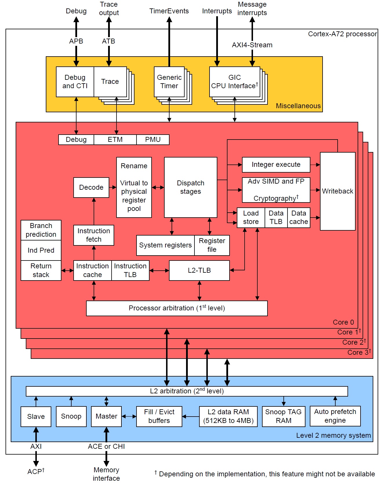
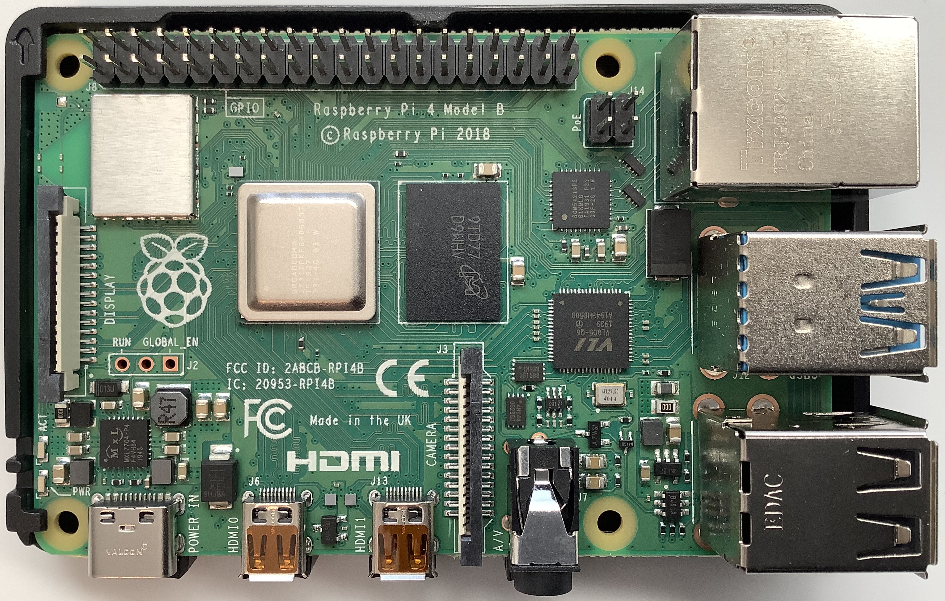
ARM architecture names have the form “ARMvX”, where X is the version number. The original Raspberry Pi (Broadcom2835 with ARM1176JZF-S processor) implemented the ARMv6 architecture. The current Raspberry Pi 4 (Broadcom BCM2711 with quad Cortex-A72 cores) implements the ARMv8-A architecture. ARMv8 is a multi-faceted beast and a short summary is wholly inadequate to convey its full scope. I suggest reading through the ARMv8 architectural profile on the ARM Web site. Suffice it to say here, ARMv8.2 is the latest.

ARMv8 was and is a big deal. ARMv7 was 32-bit only. ARMv8 took the architecture into 64-bit operation while retaining ARMv7 32-bit functionality. ARMv8 added a 64-bit ISA and operating system features, separating operation into the AArch32 execution state and the (then) new AArch64 execution state. It preserves backward compatibility with ARMv7.

You probably noticed that the core name “ARM1176JZF-S” (above) is neither the most informative nor does it suggests this core’s place in the constellation of ARM products. In 2005, ARM introduced a new core technology naming scheme. The naming scheme categorizes cores by series:

  • Cortex-A: Application
  • Cortex-R: Realtime
  • Cortex-M: Embedded

The series letters spell out “ARM” — clever. Cores within a series are tailored for their intended deployment environment having the appropriate mix of performance (speed), real estate (space) and power envelope.

The following table is a partial, historical roadmap of recent ARM cores:

    32-bit cores       64-bit cores (ARMx8) 
------------ ----------------------------------
Cortex-A5 Cortex-A53 2012 In-order LITTLE
Cortex-A7 Cortex-A57 2012 Out-of-order big
Cortex-A8 Cortex-A72 2015 Out-of-order big
Cortex-A9 Cortex-A73 2016 Out-of-order big
Cortex-A12 Cortex-A55 2017 In-order LITTLE
Cortex-A15 Cortex-A76 2018 Out-of-order big
Cortex-A17 Cortex-A77 2019 Out-of-order big

The 64-bit cores in the second column are a significant architectural break from the 32-bit cores in the first column. I will focus on the ARMv8 (64-bit) cores.

ARM rolled out big.LITTLE multiprocessor configuration at roughly the same time as ARMv8. With big.LITTLE, ARM vendors can design multiprocessors that are a mixture of big cores and LITTLE cores. LITTLE cores are power-efficient implementations much like ARM’s previous core designs for embedded and mobile systems — systems which consume and dissipate as little power as possible. Big cores trade higher power for higher performance. [If you really want to make digital electronics go fast, you must expend energy.] The big.LITTLE approach allows a mix of power-efficient cores and high-performing cores in a multicore system. Thus, a cell phone can spend most of its time in low power cores saving battery while hitting the high power cores when compute performance is required by the user.

The big.LITTLE approach is enabled by common cache and coherent communication bus design. The little guys and the big guys communicate through a common infrastructure. Nice.

ARMv8 LITTLE cores are in-order superscalar designs. In-order designs are simpler than out-of-order superscalar. In-order cores usually have a shorter pipeline, have fewer execution units, and do not require a big register file for renaming and delayed retirement. Out-of-order superscalar designs pull out all of the stops for performance and exploit as much instruction level parallelism (ILP) as they can discover.

The Cortex-A53 was the first ARMv8 in-order LITTLE core. ARM introduced its successor, Cortex-A55, in 2017.

The big core era began with Cortex-A57. This was ARM’s first design that rivaled Intel and AMD out-of-order x86 cores. The Cortex-A72 replaced the A57. Thus, the Raspberry Pi 4 (BCM2711) uses an older ARM big core, the Cortex-A72. [Explains my enthusiasm for a $70 o-o-o superscalar.] ARM have churned out new big cores on an annual basis ever since from its Austin and Sophia design centers.

Before pushing ahead, it’s worth mentioning that the Yamaha Montage synthesizer has an 800MHz Texas Instruments Sitara ARM Cortex-A8 single core processor and a 40MHz Fujitsu MB9AF141NA with an ARM Cortex-M3 core. The four 64-bit A72 cores in the Raspberry Pi 4 have much more compute throughput than the single 32-bit A8 core in the Yamaha Montage. The Montage (MODX) processor provides user interface and control and is not really a compute engine. The SWP70 silicon is the tone generator.

In practice

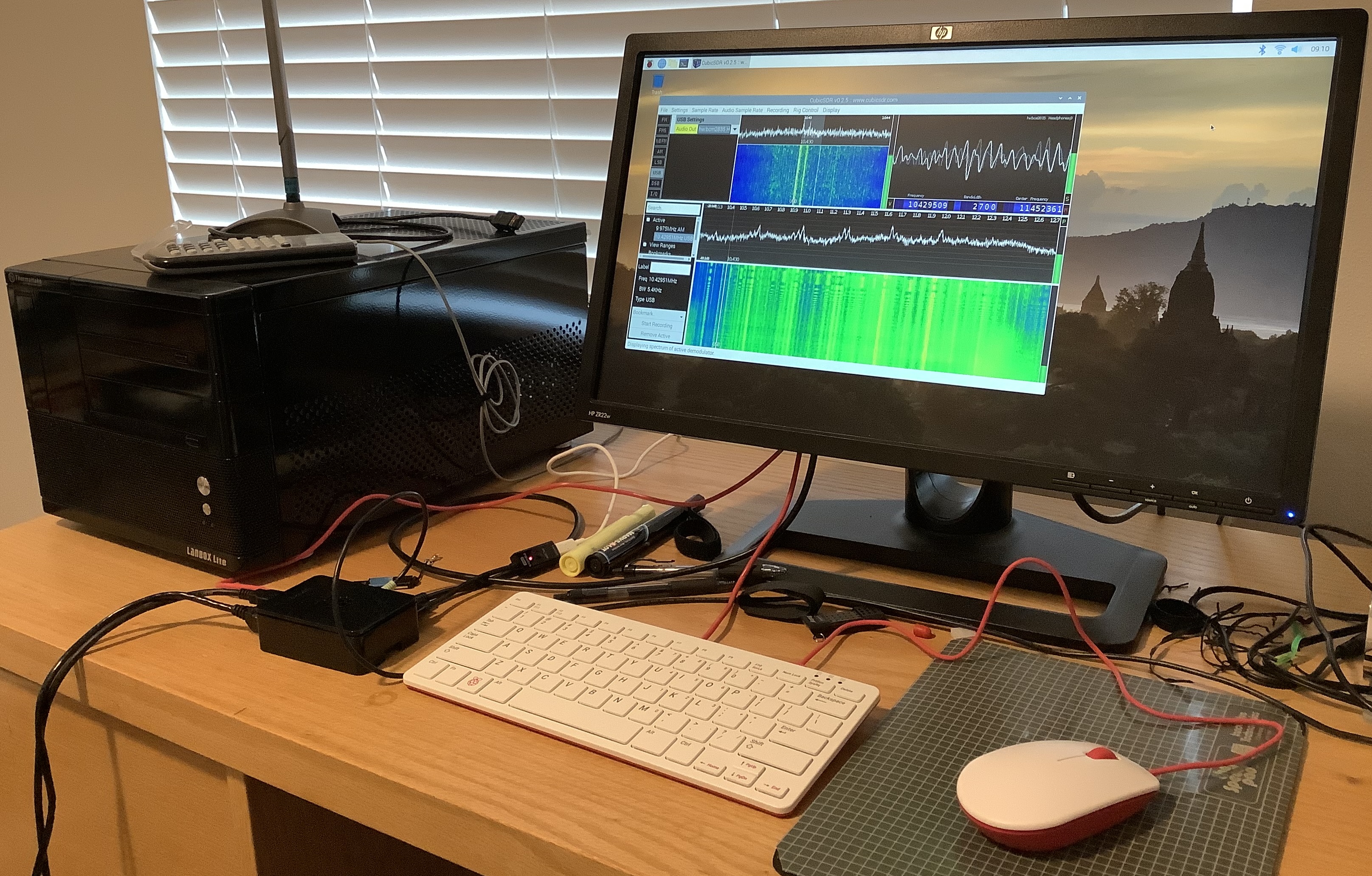
I began this dive into naming and ARM cores when I needed to determine the actual ARM core support installed with Performance Events for Linux (PERF) and the underlying kernel.

The kernel creates system files which let a program query the characteristics of the hardware platform. You might be familiar with the /proc directory, for example. There are a few such directories associated with the kernel’s performance counter interface. (See the man page for perf_event_open().) The directory:

    /sys/bus/event_source/devices/XXX/events

lists the performance events supported by the processor, XXX. In the case of the Raspberry Pi 4, XXX is “armv7_cortex_a15”. I was expecting “armv8_cortex_a72”.
Supported performance events vary from core to core. Sure, there is some commonality (retired instructions, 0x08), but there are differences between cores in the same ancestral lineage! So, one must question which default events are defined with the current version of the Raspberry Pi OS.

I found the symbolic events perf_event_open() events like PERF_COUNT_HW_INSTRUCTIONS to be reasonably sane. However, beware of the branch, TLB and L2 cache events. One must be careful, in any case, since there really isn’t a precise specification for these events and actual hardware events have many nuances and subtleties which are rarely documented. [I’ve been there.] The perf_event_open() built-in symbolic events depend upon common understanding, which is the surest path to miscommunication and misinterpetation!

Copyright © 2020 Paul J. Drongowski

Performance events on Raspberry Pi 4: Tips

Performance measurement and tuning experiments with Raspberry Pi 4 are well-underway. Here are a few quick observations and tips.

Linux provides two entries into performance measurement: Performance Events for Linux (PERF) and the kernel performance counter interface (perf_event_open()). PERF is an easy-to-use tool suite and is the best place to start explorations. If you want to measure an application without modifying its code, this is for you.

PERF is built on the kernel performance counter interface. The interface consists of two calls: perf_event_open() and its associated ioctl() functions. The kernel interface is suitable for self-monitoring, that is, adding calls to an application in order to measure its internal operation. Performance counters provide two modes of operation: counting and sampling. Counting mode is most appropriate for self-monitoring. I’m currently writing code that makes self-monitoring a bit easier and hope to post the code when it’s ready.

In the meantime…

Installation

PERF and perf_event_open support are not usually installed with your typical Linux distribution. Originally, PERF was available solely as part of the Linux tools package. Well, it seems like somewhere along the way, Ubuntu and Debian diverged. Ubuntu installs PERF with Linux tools:

    sudo apt-get install linux-tools-common 
sudo apt-get install linux-tools-common-$(uname -r)

As PERF depends heavily upon kernel facilities and interfaces, you should install the version of PERF that matches the installed kernel.

Raspberry Pi OS (once known as Raspian) is a Debian distro. Shucks, wouldn’t you know it, Debian installs PERF differently:

    sudo apt install linux-perf

There are different packages for buster and stretch (the current versions of Raspberry Pi OS and Debian at the time of this writing).

    https://packages.debian.org/buster/linux-perf 
https://packages.debian.org/stretch/linux-perf

Installing on buster produces output like:

    XXX@raspberrypi:~ $ sudo apt install linux-perf 
password for XXX:
Reading package lists… Done
Building dependency tree
Reading state information… Done
The following additional packages will be installed:
linux-perf-4.9
Suggested packages:
linux-doc-4.9
The following NEW packages will be installed:
linux-perf linux-perf-4.9
0 upgraded, 2 newly installed, 0 to remove and 107 not upgraded.
Need to get 1,275 kB of archives.
After this operation, 2,735kB of additional space will be used.
Do you want to continue? [Y/n]

Versioning gotcha

And, of course, it’s never that simple. My version of Raspberry Pi OS (buster) is expecting PERF version 5.4. When you enter “sudo perf list” or any other PERF command on the command line, the shell runs the script /usr/bin/perf. The script checks the version of PERF against the kernel and complains when versions don’t match. The Debian install pulled version 4.9, not 5.4.

Rather than sort out versioning, I’ve been entering “perf_4.9” instead of “perf“. This work-around bypasses the perf script which checks versions. Since PERF is now fairly mature, it all seems to work. At some point, I’ll sort out the versioning situation and install 5.4. In the meantime, full steam ahead!

Getting started

Here’s a few PERF commands to get you started:

    perf stat --help 
perf list sw
perf stat
perf top -a
perf top -e cpu_clock
perf record
perf report

The stat approach uses counting mode to measure software and hardware events triggered by an application program (“<cmd>”). The top approach displays event counts dynamically in real-time like the ever-popular “top” utility program. The record and report approach uses sampling to produce performance reports and profiles.

For additional usage information, check out the Linux performance analysis tutorial. There are several other fine tutorials and helpful sites on the Web. Many of the tutorials show use on x86 (Intel and AMD) systems, not Raspberry Pi and ARM. For that, I recommend my own three part tutorial:

  • Part 1 demonstrates how to use PERF to identify and analyze the hottest execution spots in a program. Part 1 covers the basic PERF commands, options and software performance events.
  • Part 2 introduces hardware performance events and demonstrates how to measure hardware events across an entire application.
    Part 3 uses hardware performance event sampling to identify and analyze hot spots within an application program.

In addition to usage, I offer information and guidance concerning ARM micro-architecture. This information is especially helpful when you get into hardware performance events. Check out my summaries of the ARM11 and ARM Cortex-A72 micro-architectures. ARM11 covers Raspberry Pi models 1, 2, and 3 (BCM2835 and BCM2836), while the Cortex-A72 summary covers the Raspberry Pi 4 (BCM2711).

Other helpful on-line resources are:

Paranoia!

Performance measurement is fraught with security issues and holes. The kernel developers implemented a control flag file, /proc/sys/kernel/perf_event_paranoid which sets the level of access and vulnerability when taking measurements. Quoting the Linux man page:

    The perf_event_paranoid file can be set to restrict access 
to the performance counters.
2 allow only user-space measurements (default since
Linux 4.6).
1 allow both kernel and user measurements (default
before Linux 4.6).
0 allow access to CPU-specific data but not raw
tracepoint samples.
-1 no restrictions.
The existence of the perf_event_paranoid file is the
official method for determining if a kernel supports
perf_event_open().

If you’re operating in a fairly closed, single-user environment, then set the content of the file to 0 or -1.

Read the perf_event_open() man page

I recommend reading the perf_event_open() man page. If you’re just starting your journey into performance measurement, you will be overwhelmed by the detail at first. However, just let the information wash over you and know that it’s there. The tutorials don’t always mention the perf_event_paranoid flag and other low-level details. Reading the man page should help you across future stumbling blocks and will enhance your understanding of events, counting and sampling.

Want to learn more about Raspberry Pi 4 (Cortex-A72 / Broadcom BCM2711) performance tuning? Please read:

Copyright © 2020 Paul J. Drongowski

Raspberry Pi 4 ARM Cortex-A72 processor

Raspberry Pi 4 (RPi4) is a big step beyond the earlier models 1, 2 and 3. Both desktop interaction and browsing are snappier and don’t have that laggy feel. I haven’t even thought (yet) about the RPi4’s music making and synthesis potential!

The Raspbeery Pi 4 is powered by a new processor from Broadcom: the BCM2711. The BCM2711 is an improvement over the BCM2835/2836 used in earlier models. Like the BCM2836, main memory is external. I’m running an RPi with 4GB of RAM (LPDDR4-3200 SDRAM, 3200Mb/s, dual channel). The old RPi2 has only 1GB of RAM. The BCM2711 supports Gigabit Ethernet (1000 BaseT) while the old RPi2 is just 100Megabit Ethernet. Faster Internet speed makes updates and browsing so much faster.

The RPi4 is a quad-core ARM Cortex-A72 processor clocking at 1.5GHz. The old RPi2 is a 900MHz quad-core ARM Cortex-A7 processor. The old BCM2835 is a member of the ARM11 family (ARM1176JZF-S, to be exact). The ARM Cortex-A72 within the BCM2711 has a much improved CPU core and memory subsystem.

The old ARM1176 is a relatively simple beast. It is a single issue machine, that is, it issues a single instruction per cycle. The ARM1176 core has eight pipeline stages and three execution pipes: 1. ALU, shift, saturation, 2. Multiply-accumulate, and 3. Load/store.

The Cortex-A72, on the other hand, performs 3-way instruction decoding and can issue as many as five operations per cycle. It is an out-of-order superscalar machine allowing speculative issue. That is waaay more sophisticated than the ARM1176, putting the Cortex-A72 on the same level as x86 superscalar machines. In fact, it translates ARM instructions into micro-ops like most modern x86 superscalar processors. It even performs micro-op fusion in some cases. The Cortex-A72 performs register renaming, letting micro-ops (instructions) execute when program data are ready (out-of-order execution, in-order retirement).

The Cortex-A72 issues micro-ops to eight execution pipelines:

  • Branch: Branch micro-ops
  • Integer 0: Integer ALU micro-ops
  • Integer 1: Integer ALU micro-ops
  • Integer Multi-Cycle: Integer shift-ALU, multiply, divide, CRC and sum-of-absolute differences micro-ops
  • FP/ASIMD 0: ASIMD ALU, ASIMD misc, ASIMD integer multiply, FP convert, FP misc, FP add, FP multiply, FP divide and crypto micro-ops
  • FP/ASIMD 1: ASIMD ALU, ASIMD misc, FP misc, FP add, FP multiply, FP square root and ASIMD shift micro-ops
  • Load: Load and register transfer micro-ops
  • Store: Store and special memory micro-ops

Up to 5-way issue and a larger number of independent execution pipelines permit more fine-grained parallelism than ARM1176. Of course, the compiler must know how to exploit all of this parallelism, but the potential is there. The ARM Cortex-A72 Software Optimization Guide specifies the number of execution cycles and pipeline units for each kind of ARM instruction. This information is incorporated into a compiler and guides the choice and scheduling of machine instructions.

ARM Cortex-A72 block diagram

The Cortex-A72 allows speculative execution. Without speculation, a CPU must wait at each conditional program branch until the direction is decided and instruction fetch can proceed along the chosen branch. The Core-A72 processor predicts branch direction (speculates) and aggressively issues instructions along predicted branches. The Cortex-A72 branch predictor is also improved over ARM1176. (I’m still digging into details.) If a branch is mispredicted, speculative results are discarded. So, it’s important to have a good branch predictor.

The Cortex-A72 can perform a load operation and a store operation every cycle because it has separate load and store pipelines. The ARMv8-A instruction set architecture (ISA) allows arbitrary data alignment and access. However, the Cortex-A72 hardware penalizes load operations that cross a cache-line (64-byte) boundary and store operations that cross a 16-byte boundary. Programmers (and compilers) should keep that in mind when laying down data structures in memory.

Like all modern high-performance computers, the Cortex-A72 organizes physical memory into a hierarchy with the fastest/smallest memory (registers) near the arithmetic/logic unit (ALU) and the slowest/largest memory (RAM) far away and off-chip. The registers and RAM are connected to intervening levels of memory — the caches:

          Register          Fast, but small 
|
Level 1 caches
|
Level 2 cache
|
RAM Big, but slow

Data and instructions are read (and written) in efficient chunks making data and instructions available when needed by the registers and ALU. The chunks are called “cache lines.” Thanks to cache memory, programs run faster when they (re)use data that are close together in memory (i.e., occupy the same cache line) and are the most recently accessed. These notions are called “spatial locality” and “temporal locality.”

The following table is a quick summary of the level 1 and level 2 cache structures of the ARM1176 and Cortex-A72.

Feature ARM1176 Cortex-A72
L1 I-cache capacity 16KB 48KB
L1 I-cache organization 4-way set associative, 32B line 3-way set associative, 64B line
L1 D-cache capacity 16KB 32KB
L1 D-cache organization 4-way set associative, 32B line 2-way set associative, 64B line
L2 cache capacity 128KB 1MB
L2 cache organization Shared, 8-way set associative, 64B line Shared, 16-way set associative, 64B line

Each core has an Instruction Cache (I-Cache) and Data Cache (D-Cache). The four cores share the Level 2 (L2) cache.

As you can see, the RPi4 (BCM2711) has larger caches and a bigger cache line size (64 bytes) than ARM11. RPi4 programs are more likely to find instructions and data in cache than earlier RPi models.

Contemporary processors have one or more memory management units (MMU) that break physical RAM into logical pages. This scheme is called “virtual memory.” The MMU translate logical program addresses (from loads, stores and instruction fetches) into physical RAM addresses. Address translation has its own memory hierarchy:

   Translation registers       Fast, but only a single mapping 
|
Level 1 TLBs
|
Level 2 TLB
|
RAM Big page tables, but slow

Page tables in RAM are maps that describe the layout of pages in the operating system and application programs. Translation lookaside buffers (TLB) are cache-like hardware structures that hold the most recently used (MRU) address translation information, i.e., where a logical page is located in physical memory. TLBs greatly speed up the translation process by keeping MRU page table information on-chip within the CPU.

Cortex-A72 has larger translation lookaside buffers (TLB) than ARM1176, as summarized in the table below. With larger TLBs, a program can touch more locations in memory without triggering a performance robbing page fault — an event which brings page translation information into the CPU from relatively slow RAM.

Feature ARM1176 Cortex-A72
D-MicroTLB capacity 10 entries 32 entries
D-MicroTLB organization Fully assoc, 1 lookup/cycle Fully assoc, 1 lookup/cycle
I-MicroTLB capacity 10 entries 48 entries
I-MicroTLB organization Fully assoc, 1 lookup/cycle Fully assoc, 1 lookup/cycle
L2 TLB capacity 256 entries 1024 entries
L2 TLB organization Unified, 2-way set assoc Unified, 4-way set assoc

Each core has a Data Micro-TLB (D-MicroTLB), Instruction Micro-TLB (I-MicroTLB), and Level 2 (L2) TLB. (In ARM1176 terminology, the L2 TLB is called the “Main TLB”).

In summary, the RPi4’s BCM2711 processor is a powerhouse even though it won’t knock that gaming machine off your desktop. 🙂 If you’ve been waiting to dive into Raspberry Pi or to upgrade, please don’t hesitate any longer.

I’m getting the itch to play with RPi4’s hardware performance counters and post results. In the meantime, check out my summary of the ARM11 micro-architecture. If you would like to know more about performance measurement and events in ARM1176-based Raspberry Pi’s, please see my Performance Events for Linux (PERF) tutorial.

Also, I have uploaded all of my teaching notes about computer design, VLSI systems and computer architecture:

These resources should help students and teachers alike!

Copyright © 2020 Paul J. Drongowski

Raspberry Pi 4 mini-review

Success with the RTL-SDR Blog V3 software defined radio (SDR) inspired me to try SDR on Raspberry Pi. I pulled out the old Raspberry Pi 2, updated to the latest Raspberry Pi OS (Buster), and installed CubicSDR and GQRX.

Both CubicSDR and GQRX ran, but performance was unacceptably slow. Audio kept breaking up, possibly due to a small audio buffer and/or insufficient CPU cycles. The poor old Raspberry Pi 2 Model B (v1.1) is a 900MHz Broadcom BCM2836 SoC, a quad-core 32-bit ARM Cortex-A7 processor. The RPi 2 has 1GB of RAM. If you would like to know more about its internals, please read about the BCM2835 micro-architecture and performance analysis with PERF (Performance Events for Linux).

Time to upgrade! I had been meaning to retire the Black Hulk — a 2011 vintage power-sucking LANbox with a Greyhound-era dual-core AMD processor. Upgrading gives me the opportunity to try the latest Raspberry Pi 4 and gain a lot of desktop space. The image below shows my office work space including the Black Hulk and the intsy RPi 4.

Raspberry Pi 4 running CubicSDR software defined radio

I decided to accessorize a little and purchased a Raspberry Pi branded keyboard and mouse. The Raspberry Pi keyboard is a small chiclet keyboard with an internal hub. The internal hub is a welcome addition and postpones the need for an external USB hub. The keyboard has a decent enough feel. It is smaller than the Logitech which it replaces, giving me more desktop space albeit with a slightly cramped hand feel. The Raspberry Pi mouse is just OK. I like the splash of color, too, a nice break from boring black and grey.

Raspberry Pi 4 is faster without question. The desktop and web browser are snappier. RPi 4 boosts the Ethernet port to 1000 BaseT (Gigabit) and you can see it.

The Raspberry Pi 4 is a 1.5GHz Broadcom BCM2711, a quad-core 64-bit ARM Cortex-A72 processor. I ran an old naive matrix multiplication program and it finished in 0.6 second versus 2.6 seconds on the Raspberry Pi 2. Naturally, I’m curious about the speed-up. I hope to dig into the BCM2711 micro-architecture.

Raspberry Pi 4 PCB (Broadcom BCM2711 and 4GB RAM)

I recommend upgrading to Raspberry Pi 4 without hesitation or reservations. I bought the Canakit PI4 Starter PRO Kit at Best Buy, not wanting to wait for delivery. The kit includes an RPi 4 with 4GB RAM, black plastic case, Canakit power supply, heat sinks, cooling fan, micro HDMI cable, USB card reader, NOOBS on a 32GB MicroSD card, and a Canakit power switch (PiSwitch). It seemed like the right combination of accessories.

By the way, you might want to consider the newly announced Raspberry Pi 400. It integrates a Raspberry Pi 4 and keyboard into one very compact unit. Its price ($70USD) is hard to beat, too.

The PiSwitch sits between the USB-C power supply and the RPi4, and is a convenient desktop power ON/OFF switch. Canakit could be a little more forthcoming about proper power up and power down sequencing. When powering down, I let the monitor go to sleep before turning power off. This should give the Raspberry Pi OS time to sync and properly shut-off.

I recommend checking the connecters on your monitor before placing any kind of web order. My HP monitor does not support HDMI, doing DisplayPort, DVI-D and VGA. The Canakit cable is micro-HDMI to HDMI. I bought a mini-HDMI to DVI-D cable on-line and wound up waiting after all! No way I’m paying Best Buy prices for a cable. 🙂

Assembly is a piece of cake. The processor and case fit together without screws or other hardware. The case fit and finish is good and holds together well just by fit alone. I installed the heat sinks, but not the fan. If I run into thermal issues, I will add the fan.

I didn’t bother with the NOOBS MicroSD card as I already had Buster installed. I see the value in NOOBS for beginners who don’t want to deal with disk images and such. I will probably repurpose the NOOBS card.

The only annoyance is due to the Raspberry Pi OS package manager. The add/remove software interface shows waaaaay too much detail. I want to install CubicSDR and GQRX, but where the heck are they? Why do I have to sort through a zillion libraries, etc. when searching on “SDR”? I installed via command line apt-get — a far more convenient and direct method.

The higher processor speed and bigger RAM pay off — no more glitchy audio. After trying both CubicSDR and GQRX, I prefer CubicSDR. I didn’t have any issues configuring for HF reception in either case. You should read the documentation (!) ahead of time, however.

I hope this quick Raspberry Pi 4 rundown is helpful.

Copyright © 2020 Paul J. Drongowski

Welcome CS teachers and students!

[Be sure to visit Living Computers in Seattle. SIGCSE 2017 attendees are admitted free during the conference. I visited the museum today and it was a lot of fun! K-12 teachers will enjoy the hands on exhibits.]

The annual ACM Special Interest Group on Computer Science Education (SIGCSE 2017) Technical Symposium is next week (March 8 – 11) in Seattle, Washington. The symposium brings together educators at all levels (K-12 and higher ed) to exchange and discuss the latest methods, practices and results in computer science education.

I don’t often advertise it, but the Sand, Software, Sound site has many resources for educators and students alike. You can browse these resources by clicking on one of the WordPress topic buttons (Raspberry Pi, PERF, Courseware, etc.) above. You can also search for a topic or choose from one of the categories listed in the right sidebar.

Here are a few highlights.

I taught many computer-related subjects during my career and have posted course notes, slides and old projects. The four main sections are:

  • CS2 data structures: Undergraduate data structures course suitable for advanced placement students.
  • Computer design: Undergraduate computer architecture and design which uses a multi-level modeling approach.
  • VLSI systems: Graduate course on VLSI architecture, design and circuits which is suitable for undergraduate seniors.
  • Topics in computer architecture: Material for a special topics seminar about computer architecture (somewhat historical).

Please feel free to dig through these materials and make use of them.

Software and hardware performance analysis formed a major thread throughout my professional life. I recommend reading my series of tutorials on the Linux PERF tool set for software performance analysis:

The ARM11 microarchitecture summary is background material for the PERF tutorial. Program profiling is a good way to bring computer architecture to life and to teach students how to analyze and assess the execution speed of their programs.

There are two additional tutorials and getting started guides for teachers and students working on Raspberry Pi:

Music technology and computer-based music-making have been two of my chief interests over the years. The Arduino section of the site has several of my past projects using the Arduino for music-making. You should also check out my recent blog posts about the littleBits synth modules and littleBits Arduino. Please click on the tags and links at the bottom of each post in order to chase down material.

You might also enjoy my tutorial on software synthesizers for Linux and Raspberry Pi. The tutorial is a getting started guide for musicians of all stripes — music teachers and students are certainly welcome, too!

5-pin MIDI IN/OUT for Arduino

I hope you enjoyed the last post about a simple tone-based sequencer for littleBits Arduino. My next goal is to make the littleBits Arduino fluent in MIDI. Then we can turn the littleBits Arduino into the heart of MIDI-based tools like real time controllers and synthesizers.

At the time of this writing, littleBits does not offer a 5-pin MIDI input module or a 5-pin MIDI output module. That shouldn’t stop us. With a little know-how and some soldering, it’s easy to whip up 5-pin MIDI IN and MIDI OUT circuits. I will show you how. Even though this discussion is in the context of littleBits Arduino, the circuits below will work with any Arduino. The circuits will even work with Raspberry Pi or Beaglebone for that matter! Once I get a couple littleBits proto modules, I’ll show you how to connect the MIDI interface circuits to the littleBits Arduino.

5-pin MIDI is a mature standard and is one of the most successful, long-running standards in personal computing. Most musicians are familier with MIDI cables and MIDI connections. MIDI cables have familiar 5-pin DIN connectors at either end. Wiring is symmetric. Unlike USB, there isn’t an A side and a B side. Connect a MIDI OUT to a MIDI IN and you’re good to go.

Even though a connector has five pins (and associated wires), only three pins are really involved in MIDI data communication. One of the three pins — “the one in the middle” — carries electrical ground. The other two pins form a current loop from the sender to the receiver and back to the sender. “Current loop” means that we are communicating 0’s and 1’s using the presence or absence of electrical current.

Everyday logic like CMOS or TTL digital circuits use voltage level to represent logical zero and logical one. Low voltage (nominally 0 Volts) represents logical zero and high voltage (nominally 5 Volts in a 5 Volt system) represents logical one. Digital circuits actually switch through a transition zone between 0 and 5 Volts. Logical 0 and 1 are defined by threshold voltages, and now we’re getting too far afield! You get the idea — the representations and electrical mode of operation are different.

Let’s start with the receiver (MIDI IN) because that’s where all of the interesting action takes place. Here is the schematic for a very basic MIDI IN. (Click on images to get full resolution.)

schematic_midi_in

The incoming current flows through a 220 ohm resistor into the optical side of a 6N138 optoisolator. That may sound scary, but Arduino folks already know how to blink an LED on and off. That’s what the current loop does. It blinks an LED in the optoisolator. The LED shines on a photodiode that controls two transistor switches. The transistors switch the output (pin 6 of the optoisolator) between logical 0 and logical 1 (in voltage-ese). Pin 6 is connected to the Arduino serial receive port (pin D0, also known as “RX”). That’s all there is to it!

The optoisolator isolates the sender and receiver electrically. This is a good thing in stage environments and any place rife with grounding problems, connection mistakes, etc. The resistor before the LED limits the current through the loop and into the LED. This resistor plus the 1N4148 diode provide input protection.

Here is the schematic for a basic MIDI OUT circuit.

schematic_midi_out

All the sender needs to do is to drive or remove an electrical current through the loop. When the loop is driven, the LED at the other end of the loop shines. When the current is removed, the LED turns off. The current loop is controlled by the Arduino send port (pin D1, also known as “TX”). The 220 ohm resistors are current limiting resistors that put a limit on the amount of current driven into the loop.

This MIDI OUT circuit gets the job, but is a little basic. Most practical commercial circuits use a driver (such as a CMOS 74HC125 buffer/driver IC) or a transistor switch. The driver provides a little more electrical assurance and protection on the sender’s side. Better to blow up an inexpensive driver IC than your Arduino!

I built both the MIDI IN and MIDI OUT circuits on an Adafruit Perma-Proto quarter-sized breadboard PCB. I like the layout of these boards and they have nice through-holes for soldering. They have the same layout as a quarter-sized solderless breadboard. In this case, you solder connections instead of inserting jumper wires and component leads into solderless breadboard holes. Please, note. If you want to use the circuits above, but are reluctant to solder, then by all means, use a solderless breadboard!

The following image shows the final result looking at the MIDI IN connector. Click the image for full resolution.

board_midi_in

The jumper wires sprouting from the board are not intended to make the board look like a court-jester. They are the connections to be made to the Arduino:

  • Red: +5 Volts
  • Black: Ground
  • Yellow: Connect to D0 / RX
  • Blue: Connect to D1 / TX

My construction style uses 2×1 and 2×2 headers to make external connections. The header pins mate up neatly with either Female/Female or Female/Male jumper wires. I used F/M jumpers in order to plug into the signal headers on a standard Arduino UNO for testing.

The next image shows the final resulting looking at the MIDI OUT connector.

board_midi_out

If you don’t mind soldering, but don’t want to go free-style on a prototyping board, then I recommend the Sparkfun MIDI Shield (DEV-12898). The latest revision of the MIDI Shield has good input protection and output drivers. It also has a RUN/PROG switch that is handy when uploading a sketch to the Arduino. MIDI and PC communications share the same serial port and conflicts must be avoided. (More about this issue in another post.) With the prototyping board, I just pull the yellow jumper wire when I upload a sketch.

The Sparkfun MIDI Shield has two knobs and three switches. This is a bonus if you are working with a standard Arduino. The knobs and switches go unused if you are working with a littleBits Arduino. In either case, the Sparkfun MIDI Shield is a viable alternative to “roll you own.”

Next time, I’ll describe the sketches that I wrote in order to test the MIDI IN and MIDI OUT.

Update: Use this simple MIDI sequencer sketch to test the MIDI OUT portion of the 5-pin interface.

We need “code-able” MIDI controllers!

All MIDI controllers for sale are rubbish!

Eh?

OK, here comes a rant. I’ve been working on two Arduino-based MIDI controllers in order to try out a few ideas for real time control. I’m using homebrew microcontrollers because I need the flexibility offered by code in order to prototype these ideas.

None of the commercial available MIDI controllers from Novation, Korg, AKAI, Alesis and the rest of the usual suspects support user coding or true executable scripts. Nada. I would love it if one of these vendors made a MIDI controller with an Arduino-compatible development interface. Connect the MIDI controller to a Mac or PC running the Arduino IDE, write your code, download it, and use it in real time control heaven! Fatal coding mistakes are inevitable, so provide an “Oops” button that automatically resets program memory and returns the unit to its factory-fresh state.

Commercial MIDI controllers have a few substantial advantages over home-brew. Commercial controllers are nicely packaged, are physically robust and do a good job of integrating keyboard, knob, slider, LED, display, etc. hardware resources into a compact space. Do I need to mention that they look good? Your average punter (like me) stinks at hole drilling and chassis building.

Commercial controllers, on the other hand, stink at flexibility and extensibility. Sure, the current crop of controllers support easy assignment of standard MIDI messages — usually control change (CC), program change (PC), and note ON/OFF. Maybe (non-)registered parameter number messages (RPN or NRPN messages) are supported. System exclusive (SysEx) most certainly is not supported other than maybe a fixed string of HEX — if you’re incredibly fortunate to have it.

The old JL Cooper FaderMaster knew how to insert control values into simple SysEx messages. This is now lost art.

Here are a few use cases for a fully user-programmable MIDI controller.

The first use case is drawbar control. Most tone-wheel clones use MIDI CC messages for drawbar control, but not all. The Yamaha Tyros/PSR “Organ Flutes” are controlled by a single SysEx message. That SysEx message sets everything at once: all the drawbar levels, percussion parameters and vibrato. Drawbar control requires sensing and sending all of the controller’s knob and switch settings in one fell swoop. None of the commercially available MIDI controllers can handle this.

If you’re interested in this project, check out these links: Dangershield Drawbars, design and code.

The second use case is to fix what shouldn’t have been broken in the first place. The Korg Triton Taktile is a good MIDI controller. I like it and enjoy playing it. However, it’s brain-damaged in crazy ways. The function buttons cannot send program change messages! Even worse, the Taktile cannot send a full program change: bank select MSB followed by bank select LSB followed by program change. This makes the Taktile useless as a stage instrument in control of a modern, multi-bank synthesizer or tone module. If the Taktile allowed user scripting, I would have fixed this nonsense in a minute.

The third use case is sending a pre-determined sequence of pitch bend messages to a tone generator. Yes, for example, you can twiddle a controller’s pitch bender wheel (or whatever) to send pitch bend. However, you cannot hit a button and send a long sequence of pitch bend messages to automatically bend a virtual guitar string or to play a convincing guitar vibrato. Punters (like me) have trouble playing good guitar articulations, but we do know how to hit buttons at the right time. Why not store and send decent sounding pitch bend and controller values in real time as the result of a simple button press?

The fourth use case is an example of the “heavy lifting” potential of user code. Many sample players and libraries (like the Vienna Symphonic Library) assign a range of keys to articulations or other methods of dynamically altering the sound of a notes played elsewhere on the keyboard (i.e., the actual melody or chord). I claim that it’s a more natural gesture to control articulations through the keyboard than to reach for a special function button on the front panel. User coding would allow the redefinition of key presses to articulations — possibly playing a different sample or sending a sequence of controller messages.

Let me give you a more specific example, which is an experiment that I have in progress. Yamaha instruments have Megavoices. A Megavoice is selected as a single patch. However, different samples are mapped to different velocity ranges and different key ranges. As such, Megavoices are nearly impossible to play through the keyboard. Nobody can be that precise consistently in their playing.

I’m prototyping a MIDI controller that implements articulation keys to control the mapping of melody notes to the individual Megavoice samples. This involves mapping MIDI notes and velocities according to a somewhat complicated set of rules. Code and scripting is made for this kind of work!

Finally, the Yamaha Montage demonstrates how today’s MIDI controllers are functionally limited. Yamaha have created excitement promoting the “Superknob” macro control. Basically, the Superknob is a single knob that — among other things — spins the parameters which have been assigned to individual small knobs. Please note “parameters” is plural in that last sentence.

Today’s MIDI controllers and their limited configuration paradigm typically allow only one MIDI message to be assigned to a knob at a time. The target VST or whatever must route that incoming MIDI value to one or more parameters. (The controllers’ engineers have shifted the mapping problem to the software developers at the other end.) Wouldn’t it be cool if you could configure a controller knob to send multiple MIDI messages at once from the source? Then, wouldn’t it be cool if you could yoke two or more knobs together into a single macro knob?

If you had user coding, you would be there already.

All site content Copyright © Paul J. Drongowski unless otherwise indicated

Tutorial: Soft synths on Linux and Raspberry Pi

Stepping back a little bit, I realized that my recent series of articles add up to a “Getting started with soft synths on Linux” tutorial. Here are the links:

I hope these articles help you, too. They are a great memory refresher for me.

Eventually, I want to turn the Raspberry Pi into a low cost, stomp box-sized, stand-alone soft synth host — kind of a cheap MIDI-driven tone module that does virtual analog synthesis. I want to run a headless Raspberry Pi — no monitor, no QWERTY keyboard, no mouse. With some clever scripting, I think it should be possible to start up the JACK audio server and a soft synth like amsynth at boot time. The soft synth would listen to a MIDI IN connected to the RPi through a standard USB MIDI interface. One possible option is to add a small touch panel (e.g., Adafruit PiTFT Plus 320×240) for simple user interaction, including system shutdown.

Qsynth and FluidSynth on Raspberry Pi: The basics

The first four articles in this series are a quick guide to getting started with audio and MIDI on Raspberry Pi 2:

  1. Get started with Raspbian Jessie and Raspberry Pi 2
  2. Get started: Linux ALSA and JACK
  3. Raspberry Pi soft synthesizer: Get started
  4. USB audio for Raspberry Pi

Although the articles address Raspbian JESSIE, the HOW-TOs should be able to get you started with pretty much any version of Linux.

I showed how to use a simple monophonic soft synthesizer (amsynth) in part 3. Now, it’s time to move on to a multi-timbral synth: FluidSynth. FluidSynth has a graphical front-end, Qsynth, and I’ll demonstrate Qsynth, too. This tutorial assumes that JACK (and/or ALSA) is properly configured. The second and third articles will help you with configuration.

The Web sites for FluidSynth and Qsynth are:

Please visit these sites to learn about the advanced capacilities that are offered by these programs. You can always consult manual pages while you are working:

    man fluidsynth
    man qsynth
    man qjackctl
    man aplay

or you can request help directly, e.g., fluidsynth --help.

Installation

Installation is a breeze:

    sudo apt-get install fluidsynth
    sudo apt-get install qsynth

These commands should automatically download and install the General MIDI SoundFont. The path name for the GM SoundFont is:

    /usr/share/sounds/sf2/FluidR3_GM.sf2

If you did not get the GM SoundFont by installing Qsynth or FluidSynth, then enter the command:

    sudo apt-get install fluid-soundfont-gm

to install it. If you want a Roland GS-compatible SoundFont, install it with the command:

    sudo apt-get install fluid-soundfont-gs

The General MIDI SoundFont file is about 140MBytes and the GS-compatible SoundFont file is about 32MBytes in size.

FluidSynth

Although you’re most likely to use FluidSynth via Qsynth, it’s worth discussing FluidSynth’s unique capabilities first. Some things can be done quite handily from the command line. The number of FluidSynth’s command line options can be overwhelming, so if you skip to Qsynth, that’s understandable.

FluidSynth is a multi-timbral software synthesizer based on SoundFont 2 specifications. It is a command line application program that accepts MIDI input from either a MIDI controller keyboard or a software MIDI sequencer. FluidSynth needs a SoundFont file containing instrument definitions and samples. It plays the incoming notes using the selected SoundFont instruments. FluidSynth supports sixteen MIDI channels (default). It provides chorus and reverb effects.

There are many SoundFonts available for download from the Web. Two of the best known and widely used SoundFonts are:

  • FluidR3_GM.sf2: A General MIDI sound set
  • FluidR3_GS.sf2: A Roland GS-compatible sound set

The General MIDI sound set is pretty good; don’t let the “General MIDI” label drive you away!

FluidSynth has three main usage modes:

  1. Interactive command mode.
  2. One-liner mode. “One-liner” is my name for this mode of operation.
  3. Server mode.

If you just type fluidsynth on the command line, FluidSynth launches into its interactive mode, i.e., FluidSynth accepts and interpets commands of its own. I won’t go into interactive mode here, but suffice it to say, that you can set parameters, load SoundFont files, etc. using FluidSynth commands. Enter help when you are in interactive mode in order to get information about commands and parameters. Interactive mode is a good way to explore FluidSynth configuration such that you can write out complicated combinations of FluidSynth command line options.

“One-liner mode” (option -i) launches FluidSynth without dropping into its interactive mode. You’re mostly likely to use this mode when launching FluidSynth from a shell script or if you just have a simple job to do from the command line.

One-liner mode means that you need to dive into FluidSynth’s command line options. There are many command line options including:

  • -C, --chorus: Turn chorus ON or OFF
  • -R, --reverb: Turn reverb ON or OFF
  • -K, --midi-channels: Set the number of MIDI channels
  • -j, --connect-jack-outputs: Connect JACK outputs
  • -F, --fast-render: Render MIDI to an audio file
  • -O, --audio-file-format: Audio file format for fast rendering
  • -r, --sample-rate: Set the sample rate
  • -T, --audio-file-type: Audio file type for fast rendering
  • -i, --no-shell: Don’t run in interative mode
  • -S, --server: Start FluidSynth as a server process

A full list of command line parameters is given in the FluidSynth User Manual.

One-liner mode handles two everyday tasks without a lot of GUI hoopla:

  1. Play back MIDI given a list of MIDI files on the command line.
  2. Render a MIDI file to an audio file (fast render).

FluidSynth looks for command line options, followed by a SoundFont file, followed by a list of MIDI files. Enter the following command to play back a MIDI file (“EvilWays.mid” in these examples) through the ALSA audio port such as the 3.5mm stereo jack on the Raspberry Pi 2:

fluidsynth -a alsa -n -i /usr/share/sounds/sf2/FluidR3_GM.sf2 EvilWays.mid

The -a option selects the ALSA audio device, -n suppresses MIDI input, and -i suppresses interactive mode. ALSA should be configured to use the 3.5mm audio jack. (See the second article in this series about ALSA and JACK.)

If you prefer to use JACK instead of vanilla ALSA, start the JACK server running via qjackctl. (See the third article in this series about using JACK with a soft synth.) Then, enter the following command:

fluidsynth -a jack -j -n -i /usr/share/sounds/sf2/FluidR3_GM.sf2 EvilWays.mid

The -a option selects JACK and the -j option tells JACK to connect the audio output of FluidSynth to the system audio output. If you leave out the -j option, JACK will not make the audio connection and you will be left wondering why there isn’t any sound coming from your speakers! You can also make this connection in the qjackctl Connections or Patchbay windows. In practice, if you aren’t getting audio output or MIDI, check your connections in JACK — audio or MIDI connections may be missing.

The image below shows the audio connection from FluidSynth to JACK. (Click on the image to enlarge it to full resolution.) This is a snapshot of the qjackctl Connections window while FluidSynth is playing a MIDI file. The audio connection is broken when FluidSynth is done with playback (i.e., when FluidSynth exits).

qjackctl_fluidsynth

Fluidsynth provides a way to fast render a MIDI file to a digital audio file. “Fast” is a relatively term. Perhaps “non-realtime render” may be a more accurate description. The following command:

fluidsynth -T wav -F EvilWays.wav /usr/share/sounds/sf2/FluidR3_GM.sf2 EvilWays.mid

converts a MIDI file (“EvilWays.mid”) to a WAV format audio file (“EvilWays.wav”). The -T option specifies the file format and the -F option specifies the name of the output file. The rendering process grinds on for a little while, so please be patient. Once you have the audio file, play it back using the ALSA aplay program:

    aplay -D hw:CODEC,0 EvilWays.wav

This example command sends digital audio to the CODEC audio device. Of course, you may use the built-in audio port or some other device. (See part 2 of this series for more examples. These tutorial articles build on each other!)

The way to get a list of audio types (-T) and audio file formats (-O) is confusing. You need to pass “help” to the appropriate command line option. (Grrrrrr.) The command:

    fluidsynth -O help

produces the following output on Raspbian JESSIE:

-O options (audio file format):
   'double','float','s16','s24','s32','s8','u8'

s8, s16, s24, s32: Signed PCM audio of the given number of bits
float, double: 32 bit and 64 bit floating point audio

The command:

    fluidsynth -T help

produces the output:

-T options (audio file type):
  'aiff','au','auto','avr','caf','flac','htk','iff','mat','mpc','oga',
  'paf','pvf','raw','rf64','sd2','sds','sf','voc','w64','wav','wve','xi'

auto: Determine type from file name extension, defaults to "wav"

Finally, server mode is needed when you want to run FluidSynth as a stand-alone server process. Qsynth is more convenient, so I won’t discuss server mode here just to keep things short.

I have to warn you, working with FluidSynth in either interactive mode or one-liner mode is not always smooth. Feedback is limited and you often have to work through rather cryptic error messages. Qsynth makes life much easier and interesting.

Qsynth

Qsynth is a graphical user interface (GUI) for FluidSynth. Qsynth is based on the Qt framework and toolset for user interface design and implementation.

Qsynth is the way to go if you want to use it as a soft synth with a MIDI controller or sequencer. It pairs up rather nicely with QJackControl, too.

We intend to demonstrate Qsynth using an M-Audio Keystation Mini 32 controller. If you’re working along with me, plug a MIDI keyboard controller into an available Raspberry Pi 2 USB port. Launch qjackctl:

    qjackctl &

and start the JACK server by clicking the Start button in the QJackCtl control panel. JACK routes the audio to the selected audio output port. Then, launch qsynth:

    qsynth

Qsynth automatically searches for the JACK server and connects audio to it. Qsynth displays a control panel which resembles an old school MIDI module. The panel knobs control master gain and the reverb and chorus effects. There are also buttons to Restart FluidSynth, to stop stuck notes (Panic), to Reset settings and to view/edit MIDI channel settings (Channels).

qsynth_panel

At this point, you need a MIDI connection from the Keystation (or other MIDI controller) to Qsynth. In the demo, I clicked the Connect button on the QJackCtl panel and made the MIDI connection using the Connections window. (See the image below. Click on the image for full resolution.)

qjackctl_qsynth

Select the Keystation entry on the left and select the FluidSynth entry on the right. Click the Connect button to make the MIDI connection. “FluidSynth” appears as a destination in the right hand column instead of “Qsynth.” Remember, Qsynth is a graphical front-end for a FluidSynth running in the background. The MIDI controller needs to communicate with the soft synth.

Play a few notes on the MIDI controller to make sure that audio and MIDI are working. Then, click the Setup button on the Qsynth front panel. Qsynth displays its Setup window which has four tabs: MIDI, Audio, Soundfonts and Settings. Click SoundFonts to go to the Soundfonts tab.

qsynth_setup

The SoundFonts tab displays the SoundFont files that are currently loaded into Qsynth (FluidSynth). Click on the Open button to load a SoundFont file like:

    /usr/share/sounds/sf2/FluidR3_GS.sf2

Use the Remove button to unload a SoundFont. Click the OK button when you are finished making changes.

If you start Qsynth with the General MIDI SoundFont and play notes on MIDI channel 1, you hear a grand piano voice. Click the Channels button on the front panel in order to change voices. With the Channels window open, double click on a row in the MIDI channel table. Should you prefer contextual menus instead, right click on a row and select Edit in the pop-up menu. This action gets you to the same place: the channel edit window (below).

qsynth_edit_channel

The channel edit window displays a list of available SoundFont voices. Voices are organized and selected in the conventional way, namely, banks and individual programs (voices). Choose a different voice like Strings (General MIDI bank 0, program 48). Qsynth does not change the voice until you click the OK button to confirm the change. If you would like to browse and try voices, check the Preview box. When Preview is enabled, Qsynth temporarily changes the voice, letting you plink away on the controller and hear the voice before changing it (or perhaps just leaving things alone by cancelling).

Click the Quit button on the Qsynth front panel when you’re finished. Then, stop the JACK server using the QJackCtl control panel.

That’s all there is to it!

Copyright © 2016 Paul J. Drongowski

USB audio for Raspberry Pi

In the first few articles of this series:

Get started with Raspbian Jessie and RPi2
Get started: Linux ALSA and JACK
Raspberry Pi soft synthesizer: Get started

we used the built-in, 3.5mm audio output from the Raspberry Pi 2 (RPi2) to produce sound through powered monitors. If you tried this with your own RPi2, you realize that the sound quality is good enough for initial experiments, but not good enough for production — unless you’re into lo-fi.

This article starts with background information about the built-in audio circuit and why it is lo-fi. Then, I briefly mention a few alternative approaches for high quality audio output and audio input. Finally, I describe my experience bringing up the Behringer UCA-202 USB audio interface on RPi2 and Raspbian JESSIE.

Built-in audio

The Raspberry Pi Foundation has not yet published a schematic for the Raspberry Pi 2. However, Adafruit (and others) claim that the audio circuit is the same as the earlier, first generation Raspberry Pi. Let’s take a look at that.

The Raspberry Pi drives a pulse width modulated (PWM) signal into a passive low pass audio filter. (See the schematic below. Click on images to enlarge and get full resolution.)

rpi_audio_schematic

The PWM technique produces OK audio, but not good, clean audio. The software performs RPDF dithering and noise shaping to improve quality. Later RPi models (like the B+ and generation 2) have better power regulation and produce less digital noise at the audio output. There is much on-line debate about further improvements, but the PWM technique seems is limited by the 11-bit quantization. (This latter point alone is subject to debate!)

JACK seems to modify the audio sample stream as well. I can hear a loud hiss from my speakers when JACK is running and sending audio through the built-in DAC circuit. Ideally, the speaker should be completely silent.

Raspberry Pi 2 does not have an audio input. Thud!

Alternatives to built-in audio

If you want better audio quality or need to record an external audio signal, there are two approaches:

  1. Buy and install an audio board.
  2. Buy and install a USB audio interface.

With respect to the first approach, I briefly explored two of the available Raspberry Pi add-on audio boards:

  1. Cirrus Logic Audio Card
  2. HiFiBerry DAC Pro+

The Cirrus Logic board is well-specified with a WM5102 audio hub, WM8804 S/PDIF transceiver, and two WM7220 digital microphone integrated circuits. Those in the know will recognize these parts as Wolfson designs. The HiFiBerry DAC+ Pro is output only and uses an equally well-respected Burr Brown digital-to-audio converter (DAC).

Potential users are advised to be careful and to check compatibility with their particular model of Raspberry Pi. Adafruit cautions that the Cirrus Logic board may not be compatible with Raspberry Pi 2.

Both boards have drivers. However, both vendors eshew device configuration and prefer to distribute full OS images that include the requisite drivers. This approach puts existing users at a disadvantage. Now that I have Raspbian JESSIE installed and running, I would like to build and install the driver by itself, not write another micro SD card and go through the bring up process again.

With these issues in mind, I decided to go the USB audio interface route. It’s also the lowest cost option for me because I already have a Behringer USB audio interface in hand.

Behringer UCA-202 audio interface

The Behringer UCA-202 is an inexpensive ($30 USD) USB audio input/output interface. Analog signals are transfered on RCA connectors (left/right IN and left/right OUT). The UCA-202 also has a headphone output and an S/PDIF optical output. The UCA-202 is bus-powered and class-compliant. Conversion is 16-bit at 32kHz, 44.1kHz or 48kHz. The UCA-202 has a sister, the UCA-222, with the same spec.

I have used the UCA-202 as a plug-and-play audio interface with both Windows and Mac OS X. Now, I can claim success with Raspbian JESSIE Linux, too. This thing is the “pocket knife” of low-cost USB audio interfaces.

Even though I’m using a Behringer UCA-202, the directions below should also apply to other class-compliant USB audio interfaces. It never hurts to search the Web for directions, problems and tips for your particular audio interface. Just sayin’.

Before plugging in the UCA-202, run aplay -l and aplay -L to see a list of the sound cards (-l) and PCMs (-L) that are installed on your machine.

Next, plug the UCA-202 into one of the USB ports. Run the aplay commands, again, and look for a new audio device. On my machine, a new sound card appears in the aplay -l output:

    card 1: CODEC [USB Audio CODEC], device 0: USB Audio [USB Audio]
      Subdevices: 1/1
      Subdevice #0: subdevice #0

The new sound card is named “CODEC”, it is ALSA card number 1, and it has one subdevice (number 0). The aplay -L output lists a whole slew of new PCMs:

    sysdefault:CARD=CODEC
        USB Audio CODEC, USB Audio
        Default Audio Device
    front:CARD=CODEC,DEV=0
        USB Audio CODEC, USB Audio
        Front speakers
    surround21:CARD=CODEC,DEV=0
        USB Audio CODEC, USB Audio
        2.1 Surround output to Front and Subwoofer speakers
    surround40:CARD=CODEC,DEV=0
        USB Audio CODEC, USB Audio
        4.0 Surround output to Front and Rear speakers
    surround41:CARD=CODEC,DEV=0
        USB Audio CODEC, USB Audio
        4.1 Surround output to Front, Rear and Subwoofer speakers
    surround50:CARD=CODEC,DEV=0
        USB Audio CODEC, USB Audio
        5.0 Surround output to Front, Center and Rear speakers
    surround51:CARD=CODEC,DEV=0
        USB Audio CODEC, USB Audio
        5.1 Surround output to Front, Center, Rear and Subwoofer speakers
    surround71:CARD=CODEC,DEV=0
        USB Audio CODEC, USB Audio
        7.1 Surround output to Front, Center, Side, Rear and Woofer speakers
    iec958:CARD=CODEC,DEV=0
        USB Audio CODEC, USB Audio
        IEC958 (S/PDIF) Digital Audio Output
    dmix:CARD=CODEC,DEV=0
        USB Audio CODEC, USB Audio
        Direct sample mixing device
    dsnoop:CARD=CODEC,DEV=0
        USB Audio CODEC, USB Audio
        Direct sample snooping device
    hw:CARD=CODEC,DEV=0
        USB Audio CODEC, USB Audio
        Direct hardware device without any conversions
    plughw:CARD=CODEC,DEV=0
        USB Audio CODEC, USB Audio
        Hardware device with all software conversions

Not all of these PCMs are defined and configured by the way. Take note of the PCM named “hw:CARD=CODEC,DEV=0”. This is essentially the raw interface to the UCA-202. This PCM, at the very least, is defined.

Connect the audio outputs of the UCA-202 to powered monitors. Test the audio output interface by playing an audio (WAV) file:

    aplay -D hw:1,0 HoldingBackTheYearsDb.wav

or:

    aplay -D hw:CARD=ALSA,DEV=0 HoldingBackTheYearsDb.wav

Please note that you need to pass in the entire PCM name “hw:CARD=CODEC,DEV=0“.

Connect an audio source to the inputs of the UCA-202. Test the audio input interface by recording to an audio (WAV) file:

    arecord -D hw:CARD=ALSA,DEV=0 -f cd test.wav

I had trouble with the duration (-d) option. YMMV. Type Control-C to stop recording. Then, play back the test audio file through the UCA-202.

That’s all there is to it! The UCA-202 is truly plug and play.

Configure JACK and other applications

You need to tell the JACK audio server to use the UCA-202 instead of the RPi’s built-in audio device. Run qjackctl and click the Settings button. Select “hw:CODEC” as the Input Device and Output Device. (See the image below.) Click OK to return to the main control panel and start the JACK server. The server routes digital audio to and from the UCA-202 and JACK clients. Launch amsynth and click its Audition button. You should hear sound from the powered monitors that are connected to the UCA-202.

qjackctl_codec

ALSA’s aplay and arecord commands are OK for testing, but are clunky for practical use. Let’s install Audacity:

    sudo apt-get install audacity

Audacity is the well-known cross-platform, open source, audio editing tool.

Edit Audacity’s preferences to set the audio interface. (See the following image.) If you want to use ALSA directly, set the interface Host to ALSA. Then set the Playback and Recording Devices to “USB Audio CODEC”. Audacity should now be able to play and record through the UCA-202.

audacity_alsa

If you prefer to use JACK instead, once again edit Audacity’s preferences. (See the following image.) Set the interface Host to “JACK Audio Connection Kit”. Set the Playback and Recording Device to “system”. Make sure the JACK audio server is running. You may need to restart Audacity at this point. Play back an audio file or try recording a new file. JACK should serve the UCA-202 audio to/from Audacity.

audacity_jack